Showing posts with label data export. Show all posts

Friday, 25 November 2022

Export cluster groups to shapefile

Biodiverse Version 4 allows users to export their cluster analyses using the same grouping process as is used to colour the branches.  

This can be convenient to reconstruct the clusters in a GIS or other graphics system.  

One issue is that only the cluster polygons (or points) are exported.  If you want to attached data from the clusters then you can export them to delimited text using the Table Grouped method (with the same grouping parameters) and use a database join to attach them to the shapefile.  The main reason for this is that shapefiles have a limit of 11 characters for field names, and many indices in Biodiverse exceed this (as well as sometimes containing characters other than letters, numbers and the underscore).  

Another point to be aware of is that each group (cell) is a separate polygon so use a dissolve to merge them if you want to remove the internal boundaries.


Pictures are better than words so here are some screenshots.  


An example cluster analysis, in this case with six clusters coloured.  

The export option is in the usual place.  It can also be accessed through the outputs tab.  


In this case the export is set to use six clusters to match the display, but you can choose whatever you like.  Other options include selecting by depth or by distance from the root (by length or depth).  


And here we have a plot of the clusters.  The colours differ but the clusters themselves are the same (and one can always update the colours).   


If you want to use the grouped clusters in a spatial condition then it is easier to do so directly - see more details here.  

If you just want to replicate the display then it is better to export the spatial data to an RGB geotiff and the tree to nexus with the colours embedded - see geotiff details here and the tree details here.  


--------


Shawn Laffan

25-Nov-2022


For more details about Biodiverse, see http://shawnlaffan.github.io/biodiverse/  


To see what else Biodiverse has been used for, see https://github.com/shawnlaffan/biodiverse/wiki/PublicationsList 


You can also join the Biodiverse-users mailing list at https://groups.google.com/group/Biodiverse-users or start a discussion at https://github.com/shawnlaffan/biodiverse/discussions 


Monday, 12 August 2019

Export cluster analyses to shapefiles

In Version 3 of Biodiverse it is possible to export your cluster and region grower analyses to shapefile formats.

This makes it easier to use the regions in geospatial analyses, for example as conditions in spatial analyses in Biodiverse.  Perhaps the best example is that you can generate a regionalisation using one data set, and then assess its values for one or more other data sets.  See for example González-Orozco et al. (2013, 2014a and 2014b).

The option is available via the export menu for cluster and region grower analyses.  The options are all the usual ones, although that is not many in this case.


The option is chosen from the export menu for a cluster (or region grower) analysis.  


There are not that many choices, but Shape type can be exported as POLYGON or POINT geometries (shapes).  You can attach lists of results, or choose to only export the geometries themselves.


You might need to run a selection to highlight the branch you are interested in.  This example is branch 120___, which corresponds to the red cluster in the first screenshot above.  You might also choose to use a Definition Query (ArcGIS) or Layer Subset (QGIS) to filter out the geometries you are not interested in.  


And here the component polygons that form the polygons for branch 120___ are highlighted in red.


There are three points to watch for.

1.  If you export a list with the data, then each polygon or point feature is repeated for each item in the list.  This is due to shapefile field names being limited to 11 characters, which is far too short for many of the list entries in Biodiverse.  (Support for the GeoPackage format is in the works to obviate this issue).

2.  The exported features (geometries) are multipolygon or multipoint.  This means that each geometry comprises one or more geometries, with each internal branch including all polygons of its terminal branches.  The internal boundaries between polygons are not dissolved, so you will see all the component polygons, but any GIS will support a dissolve operation.  If you are wondering what multipolygons and multipoints are, then Wikipedia has a decent explanation as part of the Well Known Text entry.

3.  Remember that Biodiverse knows nothing about coordinate systems and map projections (agnostic might be a better way of putting it).  You will need to define the coordinate system of the output file yourself using a GIS or other geospatial tool.


Shawn Laffan
12-August-2019

If you want to try this out before version 3 is released then the 2.99_005 development release can be accessed through the downloads page at https://github.com/shawnlaffan/biodiverse/wiki/Downloads


--------

For more details about Biodiverse, see http://shawnlaffan.github.io/biodiverse


To see what Biodiverse has been used for, see https://github.com/shawnlaffan/biodiverse/wiki/PublicationsList


You can also join the Biodiverse-users mailing list at http://groups.google.com/group/Biodiverse-users

Saturday, 22 December 2018

Visualise matrices of spatial turnover

A long standing feature in Biodiverse is the ability to interactively visualise spatial patterns of turnover.  This was described in Laffan (2011), but without detailed instructions for how to generate the data.

This blog post provides a few more details, as well as a video showing how to visualise and export the data.  Exported data can be used in, for example, NMDS analyses to relate turnover to environmental patterns (see González-Orozco et al. 2013 and González-Orozco et al. 2014).

One thing to note is that if you have a phylogeny selected then you can view which branches of the tree are shared or differ between the index and neighbour group (cell).  This is evident in the video, and is described in an earlier blog post: https://biodiverse-analysis-software.blogspot.com/2014/10/new-tree-plots-in-biodiverse.html 


1.  Generate the data


If you only want to build the matrix (or matrices) then select this option. 

2.  View the matrices

[Update 2019-01-29]  The matrix can be viewed by opening it from the Outputs tab.  The default display from the cluster analysis is the dendrogram and its associated spatial plot.

Notice the regions that become evident depending on which cells are selected.  For example, cells in South-West Western Australia are strongly related to other cells in that region, cells in Northern Australia are related across part of the top-end, while those in Tasmania extend into Victoria.


3.  Export the data


Exporting of the data is via the Export menu at the left.  It can also be done using the export button in the Outputs tab when the matrix is selected.

Currently only delimited text is supported, but you can choose whether to use normal, sparse or GDM compatible output formats.  Hovering over the options gives more details about what they do.  


Shawn Laffan

22-Dec-2018


For more details about Biodiverse, see http://shawnlaffan.github.io/biodiverse/


To see what Biodiverse has been used for, see https://github.com/shawnlaffan/biodiverse/wiki/PublicationsList


You can also join the Biodiverse-users mailing list at http://groups.google.com/group/Biodiverse-users or follow the google plus page:  https://plus.google.com/+BiodiverseSoftware


Thursday, 23 August 2018

Cluster analyses - export coloured GeoTIFF of the map to match the tree branch colours

One of the features of Biodiverse that gets the most positive feedback is the ability to colour the branches of a cluster dendrogram and then have the map show the same colours.  This makes it very easy to see where a selected cluster is, and how the clusters map spatially,

Up until now, however, it has been difficult to replicate the display without resorting to screenshots and their attendant issues with resolution (and sometimes apparent JPEG compression).

While one has been able to export the colours with the tree since version 2 was released, there was no option to match the spatial data.  With the release of version 2.1, that is now an option for the Nexus tree exports - there is a new option to export a geotiff file with associated colourmaps that can be used in GIS software.

Some images will show it best.  Below are steps to export the data and then to display it in ArcMap or in QGIS.

Note that the process works for continuous as well as discrete colour schemes.  Whatever colours were last displayed are what will be used.

This is also the process used to generate Figure 6 in Link-Pérez & Laffan (in press).

Exporting the data


An example cluster dendrogram with the associated spatial data.  It is easy to see the spatial distribution of the various clusters.  

The Nexus format is needed to export the coloured tree and geotiff, 

Be sure to select the geotiff option to get the spatial data.  If you want the tree colours as well then check that option too ("Export colours").


Displaying it in ArcMap

You need only add the raster to a data frame, as ArcMap looks for the colourmap automatically (as does ArcGIS Pro if you are using that).

ArcGIS will automatically see the colourmap file and display the colours as they were in Biodiverse.  

You can use FigTree to export the coloured tree to a PNG.  

...and display this tree in an ArcMap layout.  Note that the resolution can be an issue and you also have to convert the background to be white instead of transparent, but it often works well enough and images can be resampled to a higher resolution using most editing packages.  


Displaying it in QGIS

The QGIS process involves some manual loading of files via the layer properties dialogue.


In the Style section, set the Render type to be Singleband pseudocolor, then choose the folder icon to "load color map from file".  For a nexus file called example.nex, the colourmap file will be called example.nex.txt.   

And there it is, a display with the same colours as in Biodiverse.  


Shawn Laffan
23-Aug-2018


For more details about Biodiverse, see http://purl.org/biodiverse 


To see what Biodiverse has been used for, see https://purl.org/biodiverse/wiki/PublicationsList


You can also join the Biodiverse-users mailing list at http://groups.google.com/group/Biodiverse-users or follow the google plus page:  https://plus.google.com/+BiodiverseSoftware


Wednesday, 22 August 2018

Analysing trait data

Biodiverse is probably best known for its ability to link phylogenies to spatial data, but that's only a subset of what it can do.  It can also attach properties to each label, for example species traits like average height, seed type, locomotion method or growth form. This has been available for several versions.


Examples using label properties include colour across birds, butterflies and flowers (Dalrymple et al. 2015, 2018), plant longevity (Zhang et al. 2018), fleshiness (Chen et al. 2017), spinescence (Tindall et al. 2017) and fruit fleshiness (Rossetto et al. 2015).

The analysis of group property data has also proven useful, for example when summarising environmental conditions in bioregionalisation analyses, example González-Orozco et al. (20132014a2014b).  In these cases one assigns a value to each group (cell) to describe, for example, the mean grain size across its area.  At the moment the matching system uses exact matches on element (cell) names, so these need to be set up for the data to be correctly attached.  This can be done by importing the environmental data into Biodiverse, one layer at a time, at the same resolution and origin as the species data, and then exporting to delimited text.  The exported file will then have element names that match exactly when imported into Biodiverse as group properties.

And as a nice example that one does not need to work only with species and cells, the data in Stephenson et al. (2015) represent a spatio-temporal data set of larval herring size classes.  These are first analysed on a per-year basis across all locations, then on a per-location basis across time periods using group properties.  See the supplementary material of that article for more detailed steps. 


So how does one analyse such data using Biodiverse?  The overview is simple - one attaches the data to a BaseData object, then one analyses it.  Examples are below, followed by some other considerations like deletion, but a few concepts need to be given first.

  1. In Biodiverse, trait data are called "properties".  This is a deliberately generic term, as there is no reason why one could not analyse non-biological phenomena using the system.  (And we aim to be generic when developing Biodiverse, after all the the computer only sees numbers - it is the user who defines the analyses and interprets the results).
  2. If you are analysing trait data then you want to assign and analyse Label Property data.  This is because one can also analyse Group Properties (see below).  
  3. Both Labels and Groups are called Elements (also a more generic term), so the relevant calculations are under the "Element Properties" section of the calculation lists.  

Attaching data


This is probably best demonstrated using images of the steps with captions.

If your label property data do not match exactly, then you can use the remapping tools introduced in Version 2.

  
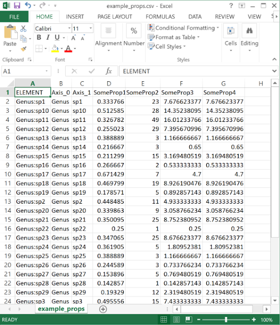
The data need to be in a delimited text (e.g. CSV format) file.  One column should match the element (label or group) name, while any number of others can be properties.  

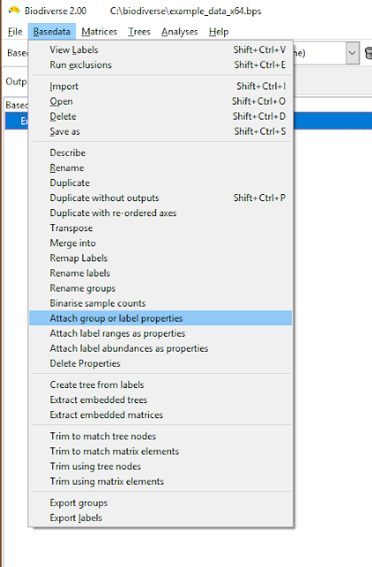
The menu option is under the Basedata menu.  

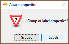
One then chooses if the properties to be assigned are for groups or labels.  In this example labels are selected.  
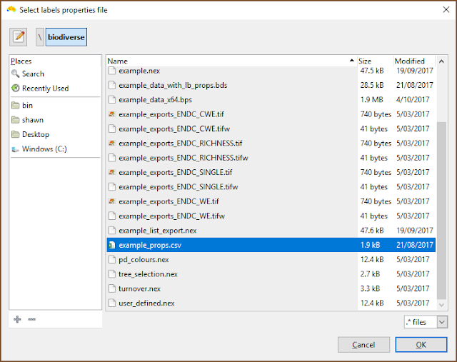
The file selection is the usual process.
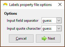
Choose the field delimiter (usually a comma) and quote character.   
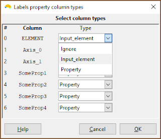
This is the important bit.  Make sure the column with the element names in it is specified as Input_element. (It does not need to be called ELEMENT).

Make sure that any column containing property data are specified as Property.  Any column with Ignore is ignored by the system.  

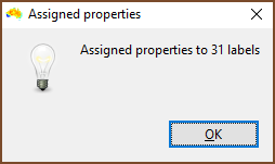
Once run, you are told how many labels or groups had properties assigned.  If there were fewer than you would expect then check the column you specified as Input_element contains matching items.  Be careful with quotes, and remember that spreadsheet programs can do odd things with your data when they import them, so use a text editor to be certain.  
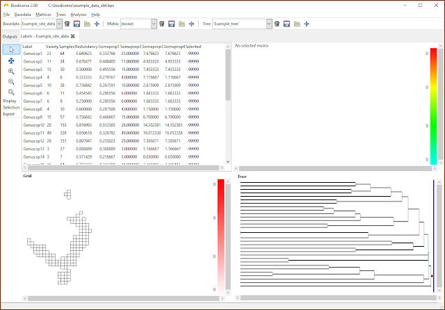
Any label properties will now be shown as additional columns in the list in the View Labels tab.

Analysing properties


Analysis of properties follows the usual process.  The example below is for a spatial analysis, but similar selections apply in the cluster and region grower analyses. 

The most important point to understand is that the results are stored as lists, and not as single scalar indices.  This make it easier to organise the results across arbitrarily named properties. 

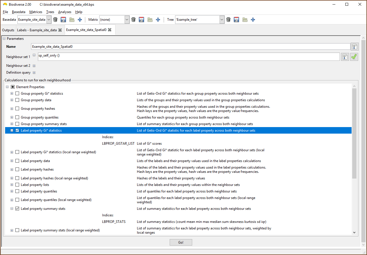
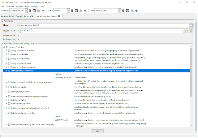
The property calculations are under the Element Properties groups in the calculations lists.  

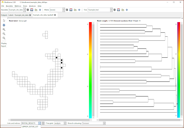
Select the list containing the desired indices.  If only property calculations have been chosen then the SPATIAL_RESULTS list will be empty.  (Note that the menu has been cropped by the screenshot in this case).  

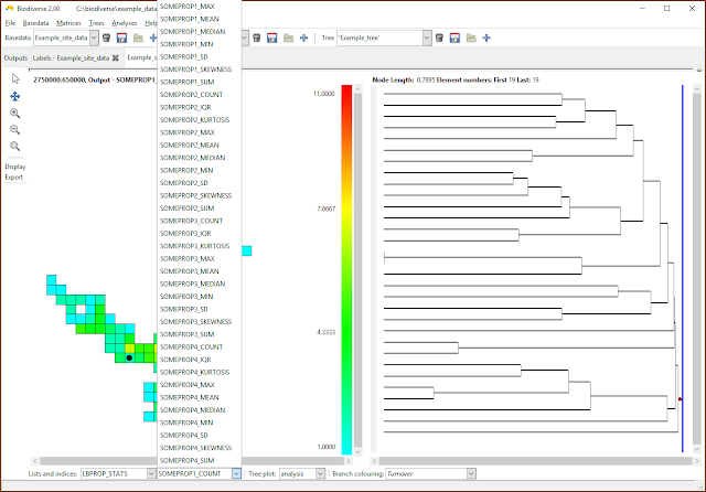
Now choose the index to be displayed.  Many of the calculations create indices in the lists that are some combination of the property name as a prefix, hence the repetition of suffixes in this example.  

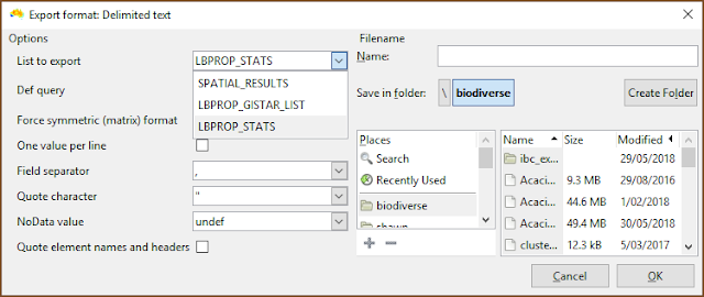
Be sure to select the desired list when exporting.


Attaching ranges and abundances 


One can also attach the label ranges and abundances as label properties, as per the next two screenshots.  Be aware, though, that these are not dynamically updated.  If you add or delete groups then these will need to be updated (unless, of course, you want the old values).


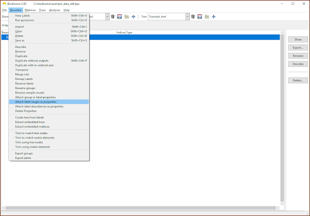
Label ranges and abundances can be attached as properties

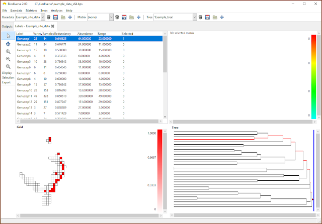
Once attached, label ranges and properties are displayed and treated just like any other property.  

It's a bit of a kludge, but if you want to attach the cell richness and sample counts for groups, then you can transpose the basedata to create a new basedata object, so the old groups are labels and the old labels are now groups.  Then attach the label ranges and abundances (remember the labels in the new object are the groups in the previous object) and transpose the data again to get back to the original structure.  This process works because the way data are stored in Biodiverse can be treated as a matrix, where the rows are the groups and the columns are the labels (consistent with many other related implementations).  The label ranges are the counts of the non-zero column entries, and the group richness scores are the counts of the non-zero row entries.  If one transposes the data then the column summations of the transposed data are on the old rows, and the same applies for the row summations. 

Can I use categories directly?

Not yet.

An implementation detail is that the property data need to be numeric, so if you have nominal classes like "gravity" or "ballistic" for seed dispersal, then you need to code them as one column each, with a value of 1 for when the trait applies, and 0 if not.  If there are unknown values then they can be left as blank and they will be ignored in the analyses.  One day we will handle categorical data.


Can I delete some of the properties after importation?  

Yes, and this has been possible since version 2 was released.

While the property import interface does not yet support column ranges (each column needs to be selected manually, which gets tedious...), one can still import more columns than are needed through inattention or because the process is automated in some way (or both). 

The deletion interface needs work, but is at least functional. There is one tab for label properties, and one for group properties. In either tab, select properties and schedule them to be deleted across all groups or labels, or choose labels and groups (elements) that will have all their property values cleared.   Nothing is actually deleted until the Apply button is pressed, and entries can be deselected.


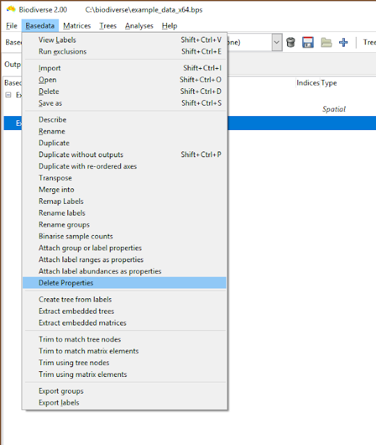
Property deletion is accessed via the Basedata menu


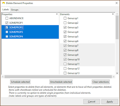
The current interface needs work, but one can select rows and then schedule those entries for deletion.  In this example, SOMEPROP1 and SOMEPROP2 will be removed from all groups, while labels Genus:sp3 to Genus:sp10 will have all their property values removed.  


It is also not possible to delete properties from a BaseData that contains outputs, even if those outputs do not use the properties.  If there is a need to do so then please raise an issue using the issue tracker.  Until it is supported, you can use the Basedata > Duplicate without outputs menu option to create a new BaseData with the same labels, groups and properties, but without any of the analysis outputs attached.  Then delete the non-required properties. 


Shawn Laffan
22-Aug-2018


For more details about Biodiverse, see http://purl.org/biodiverse 


To see what else Biodiverse has been used for, see https://purl.org/biodiverse/wiki/PublicationsList


You can also join the Biodiverse-users mailing list at http://groups.google.com/group/Biodiverse-users or follow the google plus page:  https://plus.google.com/+BiodiverseSoftware


Tuesday, 19 September 2017

Export lists to Newick format

In version 2 of Biodiverse you can now export any lists that are stored on a tree to the Nexus format.

A useful example of this is when you run calculations for each node of a cluster tree, thereby using the terminal nodes (branches) below each branch as the neighbourhood units in a spatial analysis.  An example of this in practice is in González-Orozco et al. (2014)  where the environmental parameters of each biogeographic region were summarised (see table 4 in that paper).

In a previous post I described how you can export the colours from the Biodiverse display to Nexus format to more easily generate figures for publication.  Now you can also export the values of the results to Nexus, which means you can use them for further analysis or alternate display methods using tools such as FigTree or Mesquite.

Below are images showing the general process in practice.

Note that the Nexus format does not support a hierarchy of names, so the lists need to be flattened.  Given that it is possible to have items with the same value within different lists in Biodiverse (e.g. for list indices that generate a result per label in a set), the exported names use the list name followed by the item name, joined by two underscores e.g. SPATIAL_RESULTS__ENDC_CWE.


Setting up a cluster analysis where a set of endemism indices will be calculated for each branch in the cluster tree.

Displaying the results, in this case the Corrected Weighted Endemism (CWE) for the set of branches intercepted by the blue slider bar on the dendrogram


The exported tree, but with default display settings.  


And now with thicker branches, and the colours set to show the CWE results using a divergent red-blue colour scheme.


And with the Richness index plotted using the HSB spectrum.


And here is a video of the process in Biodiverse (partly as a test to see if it works):


Shawn Laffan
19-Aug-2017


For more details about Biodiverse, see http://purl.org/biodiverse 

For the full list of changes in the 1.99 series (leading to version 2) see https://purl.org/biodiverse/wiki/ReleaseNotes (for all issues addressed or being targeted to fix for version 2, see https://github.com/shawnlaffan/biodiverse/milestone/4 ).

To see what else Biodiverse has been used for, see https://purl.org/biodiverse/wiki/PublicationsList


You can also join the Biodiverse-users mailing list at http://groups.google.com/group/Biodiverse-users


Wednesday, 26 April 2017

Constrain the extent of your exported results

This one is a short post.

Following a suggestion by Chris Barratt, Biodiverse version 2 will allow users to use a definition query when exporting spatial outputs.  This means you can run your analysis for a large data set, but limit the set of exported groups to a subset.

If the analysis itself used a definition query then the export windows will set that by default.  Just delete it to export all records.

Users can specify a definition query when exporting their data.  In this case the analysis also used a definition query so it is specified by default. 

The exported data only contain those groups (cells) that passed the definition query.  In this screenshot, no-data cells are in light grey to indicate the full extent of the exported data set.  

Shawn Laffan
26-Apr-2017


For more details about Biodiverse, see http://purl.org/biodiverse 

For the full list of changes in the 1.99 series (leading to version 2) see https://purl.org/biodiverse/wiki/ReleaseNotes (for all issues addressed or being targeted to fix for version 2, see https://github.com/shawnlaffan/biodiverse/milestone/4 ).

To see what else Biodiverse has been used for, see https://purl.org/biodiverse/wiki/PublicationsList


You can also join the Biodiverse-users mailing list at http://groups.google.com/group/Biodiverse-users