Importing group properties directly from rasters

What environmental conditions relate to my biodiversity patterns?  

Often one wants to understand which environmental conditions are associated with the taxonomic, phylogenetic and/or trait data.  Examples include edaphic and climatic variables, and publications doing so include Bickford and Laffan (2006), Gonzales-Orozco et al. (2013), González-Orozco et al. (2014a), González-Orozco et al. (2014a), Nagalingum et al. (2015) and  Bein et al. (2020).

Such data are typically obtained as rasters, with spatial resolutions often of the order of hundreds of metres.  This is in contrast to the resolution typically used for Biodiverse analyses (tens to hundreds of kilometres).

Up until now this has been something of a complex process.  The raster data need to be aggregated to the same resolution as the Biodiverse data, and aligned as part of that process.  Some sort of summary statistic needs to be calculated for each cell, usually the mean.  Then the data need to be converted to a CSV format with coordinates that exactly match the Basedata group labels so they can be attached as group properties using the import process.  The latter can be done by importing the rasters as their own basedatas, running numeric label statistics, exporting the results to CSV format and then attaching from there.  Still not simple, and not easy when there are tens of rasters to process. 

Now it is much easier

This process is greatly simplified in Biodiverse version 4, with early access via the 3.99_003 development release.  (Access to releases is via the downloads page).  

A set of rasters can be selected, imported and attached.  Biodiverse takes care of all the spatial matching and runs the summary statistics.  As a bonus, the imported data can also be attached to the project in the event the user wants to run other analyses on them.

Currently there is support for the mean, standard deviation, min, max etc.  If there is demand for other statistics like the median or inter-quartile range then these can be added.

Any raster data supported by GDAL can be imported.  Development has used geotiffs as they are the most common.  The process could probably also be generalised to support other file formats like CSV and shapefile.  It depends on demand and developer time.  

The key criteria for the raster data are that they must be in the same coordinate system as your basedata and they must represent continuous data (i.e. not be numerical categories).  The latter point is important because the group property analyses do not work with nominal/categorical values.  If you need to summarise categorical data then use an indicator approach where each class is represented by its own raster, and that raster has values of 1 for where that class occurs, and zero elsewhere.

How it works

Some screenshots are probably the best means of showing the process.  

In these examples I import two data sets from WorldClim at a 5 arc minute resolution, the Annual Mean Temperature and Mean Diurnal Range.  These are just the first two of the Bioclim layers provided by WorldClim.  The data have been projected into a Lambert Conic Conformal coordinate system to match the basedata being used (the example data that come with Biodiverse) and have been cropped to the Australian extent.

    

Annual rainfall from WorldClim2 for Australia, using a Lambert Conic Conformal projection.  Brown is low, blue is high.

The data are going to be attached to the example data that come with Biodiverse.

The process is accessed via the Basedata menu.

Rasters are selected from a folder at the same time as the options.  In this case the mean and standard deviation stats will be attached as properties to the the added to the selected basedata, and the intermediate basedatas will be added to the project so they can be visualised and/or analysed further.  

The process provides some general feedback when it completes (successfully or otherwise). 

The outputs tab shows the intermediate basedatas have been added.  Each contains a spatial analysis that was used to calculate the statistics.  

The property data cannot be visualised directly (yet).  To explore them without using an analysis you need to open the View Labels window for the basedata they were attached to and control click on a cell using your mouse.  

The popup window shows the properties for the cell that was clicked on (you will need to change the list being shown to be Properties).

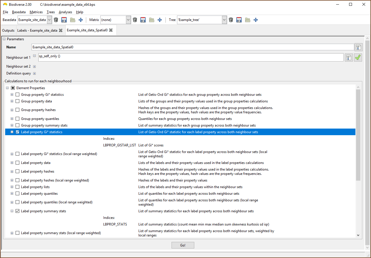
The group properties can be analysed in a spatial or cluster analysis.  Look for the calculations starting with "Group properties" under the Element Properties set.  In this case the analyses will follow those linked to the the very top and calculate summary stats and Gi* hotspot stats for each branch in a cluster tree.    

And here is a visualisation of the Gi* hotspot stat for branches cut at 0.4744 from the tips (you can slide the blue line to change this value).  The interpretation depends on your significance threshold but Gi* scores are z-scores so, for a two-tailed test where values could be high or low, values above 1.96 are hotspots at alpha=0.05, while those below -1.96 are coldspots.      

And here are the same clusters but this time coloured by the mean stat across all groups in the sample.  (The naming scheme results in lots of "means").

And here is an example of the imported raster data (diurnal range) that were used to generate the group properties.  

This image demonstrates what can happen when coarse resolution data are used.  The 5 arc minute resolution translates to approximately 18 km when projected.  The cells in the basedata containing the species observations is 50 km.  The system uses raster cell centroid coordinates to allocate their values to a basedata cell and there are clearly alignment offsets here.  There are many sources of finer resolution data you can use.    

Shawn Laffan

02-May-2022

For more details about Biodiverse, see http://shawnlaffan.github.io/biodiverse/  

To see what else Biodiverse has been used for, see https://github.com/shawnlaffan/biodiverse/wiki/PublicationsList 

You can also join the Biodiverse-users mailing list at https://groups.google.com/group/Biodiverse-users 

 

Import polygon and polyline data

The short summary: 

As of Biodiverse version 3, you can directly import polygon and polyline data from GIS feature data sets.  If you want to try it before v3 is released then it is in the current development release.

The more detailed explanation:

Ever since development started on Biodiverse it has been able to import spatial data as point records from delimited text files (e.g. CSV format).  The ability to import raster data was later added, as well as the capacity to import point records from more sources (spreadsheets and shapefiles).

However, taxon distribution records are also frequently provided in the form of polygon range maps.  One commonly used example of these are the IUCN Red List data, but there are many sources.

The way to import such data using Biodiverse 2.1 and earlier is to process the data outside Biodiverse so they can be represented as points or tables.  This is done by intersecting them with a fishnet of polygons (also called a vector grid) that aligns with the cells that will be used in Biodiverse.  Once intersected, they can be converted to points, or their coordinates added to the attribute tables, using centroid calculations.  This is what was done in López-Aguirre et al. (2018), for example.

The fishnet approach is relatively simple if one is familiar with GIS operations, but is not something that should be done by hand when numerous taxa are to be analysed or different coordinate origins are being tried.  In such cases one can script the process, but for many this can be yet another thing to learn, and not something that is done in a hurry to meet a short deadline.  (Note that scripting is a very useful skill to have, and is portable beyond the language du jour one might first learn).

With some recent changes to the Biodiverse codebase, importation of polygon data is automated and part of the standard Biodiverse data import process.  As an added bonus, polyline data are also supported, so if you have data such as for crustacean presences along stream segments then they can also be imported.

As another bonus, if you have a mix of point, line and polygon data then they can all be imported in one pass, providing they all have the fields or attributes you select.  If not then the system will throw an error.

The set of geometry attributes that are available to select from are :shape_x, :shape_y, :shape_z, :shape_m, :shape_area and :shape_length.  Not all files have all attributes.  Point files do not have a :shape_area or :shape_length, polygon files do not have :shape_length, and polyline files do not have :shape_area.  Many files do not have :shape_z or :shape_m axes - these are for 3D shapefiles or those with time measures.

A worked example

A worked example is probably the best way to show how to use it.  Those familiar with the process of importing data will note that it is almost the same as the current process, which is quite convenient in that it is one fewer thing to learn.  

Some example data.  The polygons have no specific meaning.

As usual, select the data set (or data sets) to import.  Make sure you select Shapefile as the Format.  

This step is identical to the spreadsheet and delimited text imports.

Select the fields or attributes as appropriate.  The attributes that are visible (:shape_x, :shape_m, :shape_length, :shape_area etc) depend on properties of the first file selected. 

And here is the file imported.  There is only one taxon label in this data set, so there is not much more to show, but once imported the data are analysed like any other.

How does it work?

It is essentially an automation of the process described above.

First, a fishnet grid of polygons is generated to match the cell size of the BaseData object being imported into.

There are then two ways of handling the data.

The default approach is to treat the polygon and polyline data as presence-only, so a taxon is recorded as present in any fishnet polygon that its feature data intersect with.  This is by far the fastest approach as the system can stop checking and return true as soon as it finds an intersection.

The second approach is to calculate a new data set that is the intersection of the input data set and the fishnet data set (imagine using the fishnet polygons as a cookie cutter on the taxon polygons).  This process can be substantially slower, as the system must iterate over the polygon or polyline vertices, identify where they intersect, and then cut them as appropriate. However, if you need the additional information then so be it.  That said, this approach is only used if the area or length of the intersecting features are needed, for example they are to be added as group properties or used for the sample counts.

The underlying processing is all done using the GDAL and GEOS libraries, so some of the operations will be familiar to some users as there are interfaces for Python and R, amongst other languages.

Spatial indexes 

Both approaches use spatial indexes to speed up the calculations.  As an example of the difference this makes, one data set used in testing took 9 minutes without the index, and 70 seconds with it.  For comparison, testing for presence only takes a few seconds (with the index).  It is worth noting that spatial indexes have long been used in Biodiverse to speed up processing, albeit using a different approach.

Note that, even with the spatial index, large and complex polygons will take longer to import than simple polygons.  Multipart polygons can also sometimes take longer than single part, especially if the envelope of the features (the bounding rectangle) is very large.  This is because Biodiverse needs to check all the fishnet polygons within the envelope, so if most of the fishnet polygons do not overlap the taxon polygon then most of these checks are redundant.  If there is a need then further optimisations for the above issues can be looked for.

[Update 22-12-2018 - several optimisations have since been implemented to address the above issues and will be available in the 2.99_002 development release.]

You can also just use the attribute table

There are some occasions when you only want the data from the attribute table.  If you don't use any of the geometry fields (:shape_x, :shape_area etc.) then Biodiverse will treat the table in the same way that it imports delimited text and spreadsheet data.  This means that each record in the table is the same as a row in a spreadsheet or line in a text file.

An example of when this might be useful is if you have data summarised across biomes or other regions and are not interested in analysing the data spatially, e.g. you only want to calculate Phylogenetic Diversity for the biome level assemblages and not at every location in the biome.

Shawn Laffan

10-Dec-2018

For more details about Biodiverse, see http://shawnlaffan.github.io/biodiverse/  

For the full list of changes in the 2.99 series (leading to version 3) see https://github.com/shawnlaffan/biodiverse/wiki/ReleaseNotes#version-299 (for all issues addressed or being targeted to fix for version 2, see https://github.com/shawnlaffan/biodiverse/milestone/15 ).

To see what Biodiverse has been used for, see https://github.com/shawnlaffan/biodiverse/wiki/PublicationsList

You can also join the Biodiverse-users mailing list at http://groups.google.com/group/Biodiverse-users or follow the google plus page:  https://plus.google.com/+BiodiverseSoftware

Analysing trait data

Biodiverse is probably best known for its ability to link phylogenies to spatial data, but that's only a subset of what it can do.  It can also attach properties to each label, for example species traits like average height, seed type, locomotion method or growth form. This has been available for several versions.


Examples using label properties include colour across birds, butterflies and flowers (Dalrymple et al. 2015, 2018), plant longevity (Zhang et al. 2018), fleshiness (Chen et al. 2017), spinescence (Tindall et al. 2017) and fruit fleshiness (Rossetto et al. 2015).

The analysis of group property data has also proven useful, for example when summarising environmental conditions in bioregionalisation analyses, example González-Orozco et al. (2013, 2014a, 2014b).  In these cases one assigns a value to each group (cell) to describe, for example, the mean grain size across its area.  At the moment the matching system uses exact matches on element (cell) names, so these need to be set up for the data to be correctly attached.  This can be done by importing the environmental data into Biodiverse, one layer at a time, at the same resolution and origin as the species data, and then exporting to delimited text.  The exported file will then have element names that match exactly when imported into Biodiverse as group properties.

And as a nice example that one does not need to work only with species and cells, the data in Stephenson et al. (2015) represent a spatio-temporal data set of larval herring size classes.  These are first analysed on a per-year basis across all locations, then on a per-location basis across time periods using group properties.  See the supplementary material of that article for more detailed steps. 


So how does one analyse such data using Biodiverse?  The overview is simple - one attaches the data to a BaseData object, then one analyses it.  Examples are below, followed by some other considerations like deletion, but a few concepts need to be given first.

1. In Biodiverse, trait data are called "properties".  This is a deliberately generic term, as there is no reason why one could not analyse non-biological phenomena using the system.  (And we aim to be generic when developing Biodiverse, after all the the computer only sees numbers - it is the user who defines the analyses and interprets the results).
2. If you are analysing trait data then you want to assign and analyse Label Property data.  This is because one can also analyse Group Properties (see below).  
3. Both Labels and Groups are called Elements (also a more generic term), so the relevant calculations are under the "Element Properties" section of the calculation lists.  

Attaching data

This is probably best demonstrated using images of the steps with captions.

If your label property data do not match exactly, then you can use the remapping tools introduced in Version 2.

  

The data need to be in a delimited text (e.g. CSV format) file.  One column should match the element (label or group) name, while any number of others can be properties.  

The menu option is under the Basedata menu.  

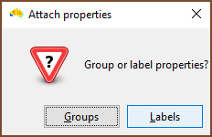
One then chooses if the properties to be assigned are for groups or labels.  In this example labels are selected.  

The file selection is the usual process.

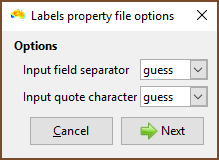
Choose the field delimiter (usually a comma) and quote character.   

This is the important bit.  Make sure the column with the element names in it is specified as Input_element. (It does not need to be called ELEMENT).

Make sure that any column containing property data are specified as Property.  Any column with Ignore is ignored by the system.  

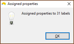
Once run, you are told how many labels or groups had properties assigned.  If there were fewer than you would expect then check the column you specified as Input_element contains matching items.  Be careful with quotes, and remember that spreadsheet programs can do odd things with your data when they import them, so use a text editor to be certain.  

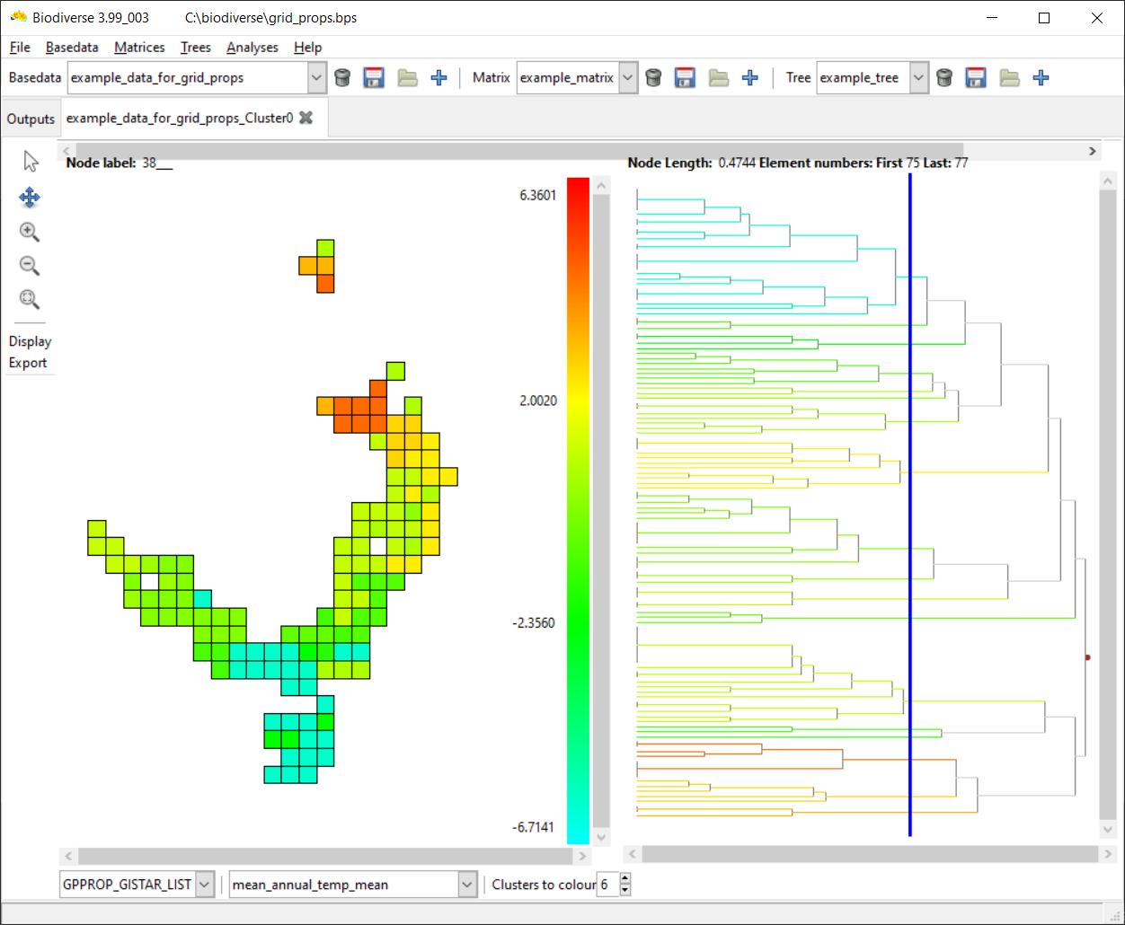
Any label properties will now be shown as additional columns in the list in the View Labels tab.

Analysing properties

Analysis of properties follows the usual process.  The example below is for a spatial analysis, but similar selections apply in the cluster and region grower analyses. 

The most important point to understand is that the results are stored as lists, and not as single scalar indices.  This make it easier to organise the results across arbitrarily named properties. 

The property calculations are under the Element Properties groups in the calculations lists.  

Select the list containing the desired indices.  If only property calculations have been chosen then the SPATIAL_RESULTS list will be empty.  (Note that the menu has been cropped by the screenshot in this case).  

Now choose the index to be displayed.  Many of the calculations create indices in the lists that are some combination of the property name as a prefix, hence the repetition of suffixes in this example.  

Be sure to select the desired list when exporting.

Attaching ranges and abundances 

One can also attach the label ranges and abundances as label properties, as per the next two screenshots.  Be aware, though, that these are not dynamically updated.  If you add or delete groups then these will need to be updated (unless, of course, you want the old values).

Label ranges and abundances can be attached as properties

Once attached, label ranges and properties are displayed and treated just like any other property.  

It's a bit of a kludge, but if you want to attach the cell richness and sample counts for groups, then you can transpose the basedata to create a new basedata object, so the old groups are labels and the old labels are now groups.  Then attach the label ranges and abundances (remember the labels in the new object are the groups in the previous object) and transpose the data again to get back to the original structure.  This process works because the way data are stored in Biodiverse can be treated as a matrix, where the rows are the groups and the columns are the labels (consistent with many other related implementations).  The label ranges are the counts of the non-zero column entries, and the group richness scores are the counts of the non-zero row entries.  If one transposes the data then the column summations of the transposed data are on the old rows, and the same applies for the row summations. 

Can I use categories directly?

Not yet.

An implementation detail is that the property data need to be numeric, so if you have nominal classes like "gravity" or "ballistic" for seed dispersal, then you need to code them as one column each, with a value of 1 for when the trait applies, and 0 if not.  If there are unknown values then they can be left as blank and they will be ignored in the analyses.  One day we will handle categorical data.

Can I delete some of the properties after importation?  

Yes, and this has been possible since version 2 was released.

While the property import interface does not yet support column ranges (each column needs to be selected manually, which gets tedious...), one can still import more columns than are needed through inattention or because the process is automated in some way (or both). 

The deletion interface needs work, but is at least functional. There is one tab for label properties, and one for group properties. In either tab, select properties and schedule them to be deleted across all groups or labels, or choose labels and groups (elements) that will have all their property values cleared.   Nothing is actually deleted until the Apply button is pressed, and entries can be deselected.

Property deletion is accessed via the Basedata menu

The current interface needs work, but one can select rows and then schedule those entries for deletion.  In this example, SOMEPROP1 and SOMEPROP2 will be removed from all groups, while labels Genus:sp3 to Genus:sp10 will have all their property values removed.  

It is also not possible to delete properties from a BaseData that contains outputs, even if those outputs do not use the properties.  If there is a need to do so then please raise an issue using the issue tracker.  Until it is supported, you can use the Basedata > Duplicate without outputs menu option to create a new BaseData with the same labels, groups and properties, but without any of the analysis outputs attached.  Then delete the non-required properties. 

Shawn Laffan

22-Aug-2018

For more details about Biodiverse, see http://purl.org/biodiverse 

To see what else Biodiverse has been used for, see https://purl.org/biodiverse/wiki/PublicationsList

You can also join the Biodiverse-users mailing list at http://groups.google.com/group/Biodiverse-users or follow the google plus page:  https://plus.google.com/+BiodiverseSoftware

Import your species data from spreadsheets

Biodiverse has always imported data from delimited text files, for example using the Comma Separated Variable (CSV) format.  Support for rasters and shapefiles (point data only) was added in version 1.  However, data is commonly collated and sent around using spreadsheets.

If one has data in a spreadsheet then, in version 1 of Biodiverse and earlier, one has to export the data from the spreadsheet to CSV format.  This rapidly becomes annoying when one is updating the spreadsheet, as one repeatedly needs to export the data.  One thing we try to avoid in developing Biodiverse is annoyance.

As of version 1.0_001, you can import spreadsheet data.  This uses the same process as for text files, except for an additional selection of the data sheet to use within the workbook.  A couple of screenshots are below to illustrate the process.  Anyone familiar with importing data into Biodiverse will note how similar it is to existing processes.

The formats supported are Microsoft Excel (.xls and .xlsx formats) and LibreOffice (.ods).

As with text files, one can import multiple spreadsheets, and the same columns will be used from each.  However, there is the limitation that the same worksheet selection will be used for all selected files.  If you have your data across multiple spreadsheets, but the structure is not consistent, then you need to repeat the import process multiple times.

You can choose to import spreadsheet files on the first page of the data import process.   

The selection options are the same as for text imports, except the rename and property options are not available.  These can be added later using the BaseData menu in the GUI.  

Select which sheet is to be used from the spreadsheet.  If you have selected multiple spreadsheets then then this selection will be applied to all of them.

The rest of the import options are the same as for text imports.  

This is the same last step in the text import process.  

This functionality is available in the 1.0_001 development release which is now available.  Please give it a try and report any success or issues.  You can do this by commenting below, or by using the mailing list or the issue tracker.  

One known problem is that the process takes a long time for large spreadsheets (300,000 rows).  In such cases it is faster to save your data to CSV format and import using the Delimited Text format.

Shawn Laffan, 22-Jun-2015

For more details about Biodiverse, see http://purl.org/biodiverse

For the full list of changes in the 1.0 series see https://purl.org/biodiverse/wiki/ReleaseNotes#version-101

To see what else Biodiverse has been used for, see https://purl.org/biodiverse/wiki/PublicationsList

You can also join the Biodiverse-users mailing list at http://groups.google.com/group/Biodiverse-users