Showing posts with label Version4. Show all posts

Wednesday, 29 March 2023

Biodiverse version 4.2 has been released


Biodiverse version 4.2 has now been released.  

Versions for Windows, Mac and Linux (Ubuntu) are available and can be accessed via https://github.com/shawnlaffan/biodiverse/wiki/Downloads


Installation instructions are at https://github.com/shawnlaffan/biodiverse/wiki/Installation


This release contains a small number of bug fixes and improved functionality. For the full list of issues and changes leading to the 4.2 release, see https://github.com/shawnlaffan/biodiverse/milestone/20

Main changes:

  • GUI
    • Branch highlighting in the View Labels tab works again. This was broken in version 4.1. Issue #850.
  • Data imports
    • Raster imports now include the band labels if defined in multiband files. Issue #852.
    • Importing a raster now works when the nodata value is NaN. Issue #851.


----

Shawn Laffan

29-Mar-2023


For more details about Biodiverse, see http://shawnlaffan.github.io/biodiverse/  


For a list of some of the analyses Biodiverse has been used for, see https://github.com/shawnlaffan/biodiverse/wiki/PublicationsList 


You can also join the Biodiverse-users mailing list at https://groups.google.com/group/Biodiverse-users or start a discussion at https://github.com/shawnlaffan/biodiverse/discussions 


Saturday, 26 November 2022

Biodiverse version 4.0 has been released

We are pleased to announce the release of Biodiverse version 4.0.  

Versions for Windows, Mac and Linux (Ubuntu) are available and can be accessed via https://github.com/shawnlaffan/biodiverse/wiki/Downloads


Installation instructions are at https://github.com/shawnlaffan/biodiverse/wiki/Installation


Version 4.0 represents 52 issues closed across 752 source code commits.  260 files have been changed.

Highlights of the changes since version 3.1 are at https://github.com/shawnlaffan/biodiverse/wiki/ReleaseNotes#version-40, and the related blog posts can be accessed via https://biodiverse-analysis-software.blogspot.com/search/label/Version4

A more detailed listing of the closed issues is at https://github.com/shawnlaffan/biodiverse/milestone/17?closed=1


-----

Shawn Laffan

26-Nov-2022


For more details about Biodiverse, see http://shawnlaffan.github.io/biodiverse/  


For a list of some of the analyses Biodiverse has been used for, see https://github.com/shawnlaffan/biodiverse/wiki/PublicationsList 


You can also join the Biodiverse-users mailing list at https://groups.google.com/group/Biodiverse-users or start a discussion at https://github.com/shawnlaffan/biodiverse/discussions 


Friday, 25 November 2022

Export cluster groups to shapefile

Biodiverse Version 4 allows users to export their cluster analyses using the same grouping process as is used to colour the branches.  

This can be convenient to reconstruct the clusters in a GIS or other graphics system.  

One issue is that only the cluster polygons (or points) are exported.  If you want to attached data from the clusters then you can export them to delimited text using the Table Grouped method (with the same grouping parameters) and use a database join to attach them to the shapefile.  The main reason for this is that shapefiles have a limit of 11 characters for field names, and many indices in Biodiverse exceed this (as well as sometimes containing characters other than letters, numbers and the underscore).  

Another point to be aware of is that each group (cell) is a separate polygon so use a dissolve to merge them if you want to remove the internal boundaries.


Pictures are better than words so here are some screenshots.  


An example cluster analysis, in this case with six clusters coloured.  

The export option is in the usual place.  It can also be accessed through the outputs tab.  


In this case the export is set to use six clusters to match the display, but you can choose whatever you like.  Other options include selecting by depth or by distance from the root (by length or depth).  


And here we have a plot of the clusters.  The colours differ but the clusters themselves are the same (and one can always update the colours).   


If you want to use the grouped clusters in a spatial condition then it is easier to do so directly - see more details here.  

If you just want to replicate the display then it is better to export the spatial data to an RGB geotiff and the tree to nexus with the colours embedded - see geotiff details here and the tree details here.  


--------


Shawn Laffan

25-Nov-2022


For more details about Biodiverse, see http://shawnlaffan.github.io/biodiverse/  


To see what else Biodiverse has been used for, see https://github.com/shawnlaffan/biodiverse/wiki/PublicationsList 


You can also join the Biodiverse-users mailing list at https://groups.google.com/group/Biodiverse-users or start a discussion at https://github.com/shawnlaffan/biodiverse/discussions 


Trees: Merge single-child branches with their children

When Biodiverse is used to trim a tree to a subset of branches, for example to match the selected BaseData object, any branch with no remaining descendants is removed from the tree.  All other branches are retained.  

What this means is that some internal branches (nodes) can be left with only one child branch (node),.  These can be referred to as single-child nodes and also knuckles.  Retaining such nodes can be useful if some of the structure of the original tree needs to be kept, for example to indicate that there is phylogenetic data but that it has been removed from the tree.  The counter to this is that most phylogenetic trees are samples and so are likely to be missing many branches anyway.

In the spirit of letting the user decide, Biodiverse version 4 supports the merger of internal branches with their children if they have only one child. 

Names are important, and like many systems any node can be named in Biodiverse.  In fact, all nodes have names but internal nodes default to a number with three trailing underscores (so "1___", "35___" etc).  This allows many of the branch and clade level indices such as the phylogenetic endemism clade contributions and PD clade loss.  

The general rule when merging is that the name of the merged node is whichever node had a non-default name to begin with.  If both have non-default names then a child that is a terminal wins.  Otherwise the parent name is used.  

The process is best demonstrated using images.  


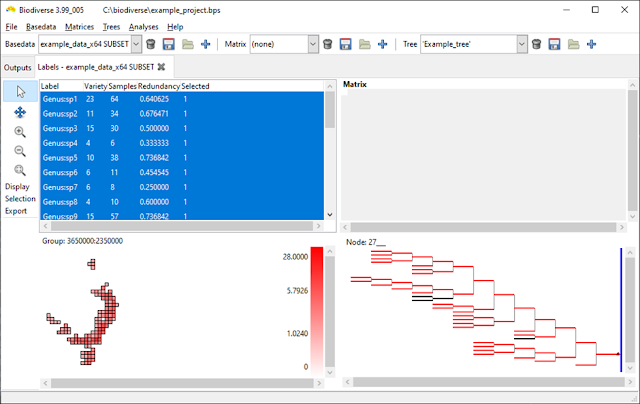
An example tree plotted using depth instead of length to show the individual branches.  The black branches are not in the basedata.  

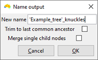
The tree trimming interface includes the option to merge single child nodes.  In this case it is not selected.   


The black branches from the previous screenshot have been deleted but one can see several branches that appear twice as long as the others. These are actually pairs of branches.


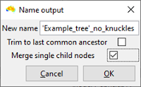
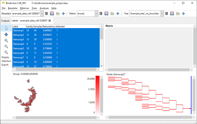
Repeating the process above but this time merging the single child (knuckle) nodes.  


In this case all the branches are the same length because all single child branches have been merged with their children.  


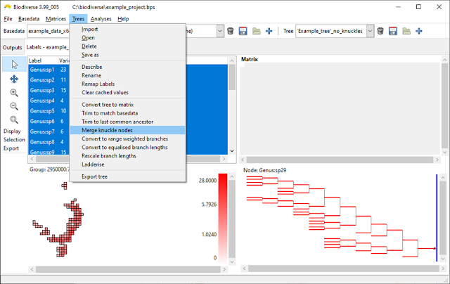
The examples above all use the tree trimming process, but if you have a tree that already has knuckles or forget to merge them then you can also merge the nodes directly from the tree menu.  


Direct access to the merging process.  

--------

Shawn Laffan

25-Nov-2022


For more details about Biodiverse, see http://shawnlaffan.github.io/biodiverse/  


To see what else Biodiverse has been used for, see https://github.com/shawnlaffan/biodiverse/wiki/PublicationsList 


You can also join the Biodiverse-users mailing list at https://groups.google.com/group/Biodiverse-users or start a discussion at https://github.com/shawnlaffan/biodiverse/discussions 


Tuesday, 25 October 2022

Biodiverse now calculates CANAPE for you

The CANAPE protocol is one of the analyses Biodiverse is most commonly used for (see examples amongst the list of publications using Biodiverse).  

The method, or protocol, was originally described in Mishler et al. (2014) and is conceptually simple.  Run an analysis that includes phylogenetic endemism and relative phylogenetic endemism, run those through a randomisation, and then categorise the results based on the significance score of the indices.  This process is described in more detail in previous posts here and here.  

The main issue with the approach to date is that the CANAPE classes are determined outside of Biodiverse using systems like a GIS, R code or a spreadsheet.  So while the process is conceptually simple, the actual implementation can all get a bit complex. Many users are not entirely sure which indices to pass through their functions, or even which lists to extract them from.  

As of Version 4 Biodiverse now calculates it for you.  This occurs automatically whenever an analysis has included the Phylogenetic Endemism and Relative Phylogenetic Endemism type 2 calculations.   (If you want it sooner than version 4 then it is in the development release 3.99_005, which was current at the time of writing.  See the downloads page for links).


Biodiverse now calculates the CANAPE scores when the requisite indices have been calculated, and a randomisation has been run.  Like many of the posts on this blog, this example uses the Acacia data set from Mishler et al. (2014).

How does Biodiverse store the results? 

The results are stored in a new list where the name is the randomisation output used followed by ">>CANAPE>>".  So for a randomisation called "rand" you would see "rand>>CANAPE>>".  The use of angle brackets might look a bit strange at first but makes the naming consistent with the other randomisation lists and simplifies the underlying code.

The CANAPE classes are stored in an index called CANAPE_CODE, with a numeric code indicating which of the categories a cell falls in.  Currently this code is 0 for not significant, 1 for neo-endemism, 2 for palaeo-endemism and 3 for mixed endemism.

Biodiverse also provides individual indices for neo, palaeo and mixed in the event a user only wants to see which cells are are in a specific class.  For example one might want to run a cluster analysis using only neo-endemism cells following the process described here.  


The same data as above but highlighting Palaeo-endemism cells in red.  All other cells containing data are in blue.  


Visualisation

A big advantage of generating CANAPE results within Biodiverse is that users can now explore the results using the functionality Biodiverse provides.  As an example, the next screen shot shows an exploration of the contribution of each clade on the tree in relation to the analysis groups (cells) (see more details about that process here and here).  

Each tree branch is coloured by the relative contribution of the clade subtending it to the PE score in the cell being hovered over (black dot in south-western WA).  This allows an understanding of which clade is driving the PE scores, and thus CANAPE, in a cell.  The visualisation process is explained in more detail here.  


Displaying the results in other systems

If you then want to use the plots as part of a map then they can be exported to an RGB Geotiff.  Details of how to do this are in another post but the next two screenshots show the start and end.  


What about a different colour scheme?


The colour scheme used is from Mishler et al. (2014) where neo is red (new is hot), palaeo is blue (old is cold) and purple is between blue and red on a colour wheel.  

If you prefer a different colour scheme then you can export the data as you normally would, for example as CSV files or as non-RGB geotiffs, and recreate the plot to your own tastes.  

Changing the colours within Biodiverse would be very useful and contributions are always welcome.

What about the Super class?  


The system does not currently generate the Super class.  It can be added if there is demand.  (Edit: It was added for Biodiverse Version 5).

Do I have to run a new randomisation analysis to see the CANAPE list?  


The CANAPE lists are generated at the end of any sequence of randomisations.  If you already have a randomisation analysis then they can be created by running one additional iteration.  

If you are concerned that your analysis is already at 999 iterations then all you lose is a bit of numeric neatness as there are now 1001 realisations in total instead of 1000 (one original plus all the random ones).  This is unlikely to make any meaningful difference once that many iterations have been run.

--------

Shawn Laffan

25-Oct-2022


For more details about Biodiverse, see http://shawnlaffan.github.io/biodiverse/  


To see what else Biodiverse has been used for, see https://github.com/shawnlaffan/biodiverse/wiki/PublicationsList 


You can also join the Biodiverse-users mailing list at https://groups.google.com/group/Biodiverse-users or start a discussion at https://github.com/shawnlaffan/biodiverse/discussions 


Sunday, 10 July 2022

Biodiverse now calculates indices for the variation in phylogenetic distinctness

Biodiverse has included calculations of indices from the phylocom system for several versions, specifically the Mean Phylogenetic Distance (MPD) and Mean Nearest Taxon Distance (MNTD).  The MPD is the average of the pair-wise distances between tree tips in a sample, where the distances pass through all the shared ancestors below the most recent common ancestor.  The MNTD is the average distance for each tip to its nearest tip in the sample.

There are many ways of slicing and diving a sample, and one of the development principles of Biodiverse is to provide more details rather than less.  Consequently there are also indices for the pair-wise root mean standard deviation (RMSD), minimum and maximum distances between a sample of tips on a tree.   

The min and max are simply the longest and shortest distances in the pairwise sample, so the distances between the most and least related pairs.  The RMSD is the square root of the mean squared distance and is a measure of the variability in a sample. It is analogous to a standard deviation but where the expected value (the mean) is zero, and follows the same formulation as the Root Mean Squared Error except a value of zero in RMSE means no error whereas in RMSD it means a zero distance between tips on the tree. 

However, the RMSD is not the variance and sometimes one is looking to see how a set of pair-wise distances is distributed around the mean.  This is where the Variance becomes useful, as first described by Warwick and Clarke (2001).

Biodiverse version 4 includes indices for the variance of the pairwise distances.  The index names are subject to change before then but for now follow the pattern PMPD1_VARIANCE, PMPD2_VARIANCE and PMPD2_VARIANCE, where the 1, 2 and 3 indicate unweighted (each tip counts equally), locally range weighted (tips count as many groups they occur in the neighbourhood) and locally abundance weighted (using the number of samples of each tip in the neighbourhood).  These are calculated by default when the relevant MPS and MNTD indices are requested. 

The variance indices are calculated with the other MPD and MNTD indices.  

Plotting is the same as for any index.  Some cells are blank because values are undefined when the sample contains only one tip, and therefore no path between tips.  Zero variances are where there are only two tips, and thus no variation.  


This is just a plot of the mean for comparison.  


But are the values significant?

A common approach to testing significance of the MPD and MNTD indices in the unweighted case is to use a resampling approach.  For each sample this generates a distribution of possible values under random resampling of the same number of tips.  More details are given in another blog post.  

The unweighted pairwise variance is also assessed in this way, with the index name using NET_VPD.  As with NRI and NTI, this is a z-score so values more extreme than +/-1.96 can be considered significantly higher or lower than expected.  

The resampling approach uses the same code as for NRI and NTI so the same sequence of resamples can be used across NRI, NTI and NET_VPD, although in Biodiverse version 4 this is only for NTI for non-ultrametric trees an exact calculation is used for NRI with any trees and for NTI for ultrametric trees.  This exact calculation avoids resampling and is much faster to run.  More details and references are in the same blog post referred to above).

The NET_VPD indices are also under the PhyloCom set.  Users can calculate the NET_VPD as well as the expected values used in its calculation.  


Values are z-scores.  At least three tips are needed to calculate the z-score as standard deviations are always zero for two tips and thus the z-score is undefined.


Control clicking on cells allow users to see the values for all indices that were calculated (within each output list, where SPATIAL_RESULTS is where most go).   


Shawn Laffan

10-Jul-2022


For more details about Biodiverse, see http://shawnlaffan.github.io/biodiverse/  


To see what else Biodiverse has been used for, see https://github.com/shawnlaffan/biodiverse/wiki/PublicationsList 


You can also join the Biodiverse-users mailing list at https://groups.google.com/group/Biodiverse-users or start a discussion at https://github.com/shawnlaffan/biodiverse/discussions 


Monday, 2 May 2022

Use clusters in spatial conditions

Spatial conditions are a core part of Biodiverse

Most people seem to focus on using single cells for their analysis and trying to find the ideal cell size.  This is missing much of the benefit of spatial analyses.  You are not constrained to using single cells in isolation.  

You can analyse regions around each focal location (processing group) using geometric shapes like circles.  Varying the size of the window gives an understanding of the spatial scale of the patterns (the operational scale).  However, there is no need to be geometric - you can use arbitrarily complex spatial conditions based on polygon features, proximity and/or matching text.  See for example Laffan and Crisp (2003) and Laity et al. (2015).  

You can also use cluster (and region grower) analyses to define your spatial windows.  These allow you to let the data define the regions, with the calculations then applied giving you more understanding of the groupings that have been identified.  Care needs to be taken with interpretation due to the risk of circularity, but that's not unusual.  And sometimes you just want to understand something about the assemblage that falls under a node (branch).  You might also be interested in the environmental properties associated with a cluster.

One issue with the cluster approach is that it can be difficult to use the branches in a spatial condition for a different analysis.  Consider the case where one wants to spatially partition a randomisation so labels are kept within their associated clusters (for a given cluster cutoff).  You could export the clusters to shapefile format, extract the relevant features to a new shapefile, and then use that in a new spatial condition.  But that's a lot of work and not easy for people less familiar with geoprocessing and GIS.  

From version 4 you can access the set of groups under a cluster analysis and use that to define spatial conditions (actually it is in the 3.99_003 development version).  This can use any of the current cutting methods, so you can slice by distance from the tips, depth, or number of clusters from the root using the sp_points_in_same_cluster condition.  You can also select individual branches (nodes) by name (sp_point_in_cluster).   

Some snippets are below that can be copied into your spatial conditions windows.  No screenshots this time, but I can add a new post of that is needed.  

Note that the cluster analysis being referred to must be in the same basedata.  


## sp_points_in_same_cluster examples

#  Try to use the highest four clusters from the root.
#  Note that the next highest number will be used
#  if four is not possible, e.g. there might be five
#  siblings below the root.  Fewer will be returned
#  if the tree has insufficient tips.
sp_points_in_same_cluster (
  output       => "some_cluster_output",
  num_clusters => 4,
)

#  Cut the tree at a distance of 0.25 from the tips
sp_points_in_same_cluster (
  output          => "some_cluster_output",
  target_distance => 0.25,
)

#  Cut the tree at a depth of 3 from the root.
#  The root is depth 1.
sp_points_in_same_cluster (
  output          => "some_cluster_output",
  target_distance => 3,
  group_by_depth  => 1,
)

#  Select four clusters below a specified node
sp_points_in_same_cluster (
  output       => "some_cluster_output",
  num_clusters => 4,
  from_node    => '118___',  #  use the node's name
)

#  target_distance is ignored if num_clusters is set
#  so this is the same as the first example
sp_points_in_same_cluster (
  output          => "some_cluster_output",
  num_clusters    => 4,
  target_distance => 0.25,
)


## sp_point_in_cluster examples

#  This will select any element that is a terminal in the cluster output
#  It is useful when the cluster analysis was run under
#  a definition query to reduce the number of elements clustered,
#  and you want the same set of elements.
sp_point_in_cluster (
  output       => "some_cluster_output",
)

#  Now specify a cluster within the output
sp_point_in_cluster (
  output       => "some_cluster_output",
  from_node    => '118___',  #  use the node's name
)

#  Specify an element to check instead of the current
#  processing element.
sp_point_in_cluster (
  output       => "some_cluster_output",
  from_node    => '118___',  #  use the node's name
  element      => '123:456', #  specify an element to check
)


Shawn Laffan

02-May-2022


For more details about Biodiverse, see http://shawnlaffan.github.io/biodiverse/  


To see what else Biodiverse has been used for, see https://github.com/shawnlaffan/biodiverse/wiki/PublicationsList 


You can also join the Biodiverse-users mailing list at https://groups.google.com/group/Biodiverse-users 


Importing group properties directly from rasters

What environmental conditions relate to my biodiversity patterns?  

Often one wants to understand which environmental conditions are associated with the taxonomic, phylogenetic and/or trait data.  Examples include edaphic and climatic variables, and publications doing so include Bickford and Laffan (2006), Gonzales-Orozco et al. (2013), González-Orozco et al. (2014a), González-Orozco et al. (2014a), Nagalingum et al. (2015) and  Bein et al. (2020).

Such data are typically obtained as rasters, with spatial resolutions often of the order of hundreds of metres.  This is in contrast to the resolution typically used for Biodiverse analyses (tens to hundreds of kilometres).

Up until now this has been something of a complex process.  The raster data need to be aggregated to the same resolution as the Biodiverse data, and aligned as part of that process.  Some sort of summary statistic needs to be calculated for each cell, usually the mean.  Then the data need to be converted to a CSV format with coordinates that exactly match the Basedata group labels so they can be attached as group properties using the import process.  The latter can be done by importing the rasters as their own basedatas, running numeric label statistics, exporting the results to CSV format and then attaching from there.  Still not simple, and not easy when there are tens of rasters to process. 

Now it is much easier

This process is greatly simplified in Biodiverse version 4, with early access via the 3.99_003 development release.  (Access to releases is via the downloads page).  

A set of rasters can be selected, imported and attached.  Biodiverse takes care of all the spatial matching and runs the summary statistics.  As a bonus, the imported data can also be attached to the project in the event the user wants to run other analyses on them.

Currently there is support for the mean, standard deviation, min, max etc.  If there is demand for other statistics like the median or inter-quartile range then these can be added.

Any raster data supported by GDAL can be imported.  Development has used geotiffs as they are the most common.  The process could probably also be generalised to support other file formats like CSV and shapefile.  It depends on demand and developer time.  

The key criteria for the raster data are that they must be in the same coordinate system as your basedata and they must represent continuous data (i.e. not be numerical categories).  The latter point is important because the group property analyses do not work with nominal/categorical values.  If you need to summarise categorical data then use an indicator approach where each class is represented by its own raster, and that raster has values of 1 for where that class occurs, and zero elsewhere.

How it works

Some screenshots are probably the best means of showing the process.  

In these examples I import two data sets from WorldClim at a 5 arc minute resolution, the Annual Mean Temperature and Mean Diurnal Range.  These are just the first two of the Bioclim layers provided by WorldClim.  The data have been projected into a Lambert Conic Conformal coordinate system to match the basedata being used (the example data that come with Biodiverse) and have been cropped to the Australian extent.


Annual rainfall from WorldClim2 for Australia, using a Lambert Conic Conformal projection.  Brown is low, blue is high.

The data are going to be attached to the example data that come with Biodiverse.

The process is accessed via the Basedata menu.

Rasters are selected from a folder at the same time as the options.  In this case the mean and standard deviation stats will be attached as properties to the the added to the selected basedata, and the intermediate basedatas will be added to the project so they can be visualised and/or analysed further.  

The process provides some general feedback when it completes (successfully or otherwise). 

The outputs tab shows the intermediate basedatas have been added.  Each contains a spatial analysis that was used to calculate the statistics.  

The property data cannot be visualised directly (yet).  To explore them without using an analysis you need to open the View Labels window for the basedata they were attached to and control click on a cell using your mouse.  


The popup window shows the properties for the cell that was clicked on (you will need to change the list being shown to be Properties).

The group properties can be analysed in a spatial or cluster analysis.  Look for the calculations starting with "Group properties" under the Element Properties set.  In this case the analyses will follow those linked to the the very top and calculate summary stats and Gi* hotspot stats for each branch in a cluster tree.    

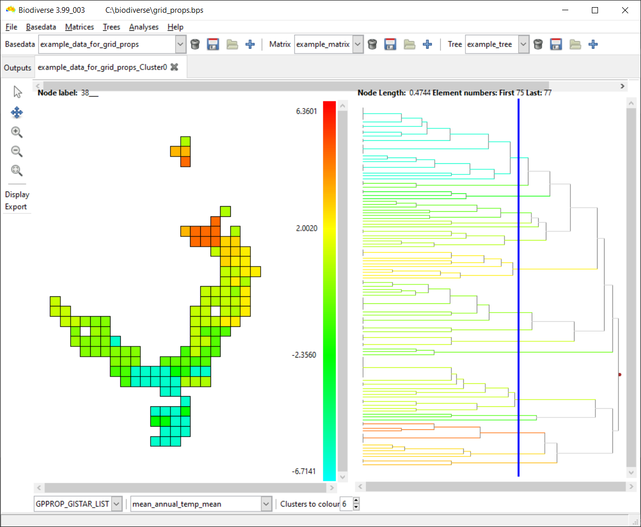
And here is a visualisation of the Gi* hotspot stat for branches cut at 0.4744 from the tips (you can slide the blue line to change this value).  The interpretation depends on your significance threshold but Gi* scores are z-scores so, for a two-tailed test where values could be high or low, values above 1.96 are hotspots at alpha=0.05, while those below -1.96 are coldspots.      

And here are the same clusters but this time coloured by the mean stat across all groups in the sample.  (The naming scheme results in lots of "means").

And here is an example of the imported raster data (diurnal range) that were used to generate the group properties.  

This image demonstrates what can happen when coarse resolution data are used.  The 5 arc minute resolution translates to approximately 18 km when projected.  The cells in the basedata containing the species observations is 50 km.  The system uses raster cell centroid coordinates to allocate their values to a basedata cell and there are clearly alignment offsets here.  There are many sources of finer resolution data you can use.    


Shawn Laffan

02-May-2022


For more details about Biodiverse, see http://shawnlaffan.github.io/biodiverse/  


To see what else Biodiverse has been used for, see https://github.com/shawnlaffan/biodiverse/wiki/PublicationsList 


You can also join the Biodiverse-users mailing list at https://groups.google.com/group/Biodiverse-users 


Friday, 24 September 2021

Faster calculation of PhyloCom indices: NRI, NTI, MPD and MNTD

This post covers a bit more of the internals than we usually do.  Hopefully it is useful.  

From version 4, Biodiverse will use faster methods to calculate the indices in the PhyloCom set, with ultrametric trees seeing the greatest speedup.  These are the NRI, NTI, MPD and MNTD indices, which when not "acronymed" are the Net Related Index, the Nearest Taxon Index, Mean Phylogenetic Distance and Mean Nearest Taxon Distance.  These were originally implemented in the phylocom software (Webb et al. 2008) and many readers will be familiar with the R package picante.  

The MPD index is a measure of the mean of the paths along the tree between each pair of tips in a sample.  The contribution of a branch is proportional to its length and the number of paths it is part of.  

The MNTD index is the mean of the shortest path between each tip in a sample and the nearest tip that is also in the sample.  For a sample of ten tips there are only ten paths, but in the naïve case one needs to evaluate all paths to determine which is the shortest.  

One point to keep in mind is that branches in MPD and MNTD are counted one or more times, more specifically as many paths that they form part of.  This is in contrast with PD where each branch counts only once.  The number of paths also increases quadratically with the number of tips in the sample.  For example, if there are ten tips then there will be 10*(10-1)/2=45 paths to connect all pairs, and if there are 10,000 tips then there are 49,995,000 paths.  To my mind these make PD a better index, but that discussion is for another day.  Certainly it is simpler to calculate.

The NRI and NTI are z-scores of the MPD and MNTD scores, respectively, and indicate if the paths are longer or shorter than expected given a random resampling of tips across the tree.  The resampling algorithm can vary, but the simplest is to use the same number of tips as is found in the sample. In other words it matches the richness of the observed sample, so if one has ten tips in an observed sample then each random iteration draws ten tips at random and calculates the MPD and MNTD score.  There are other random sampling algorithms, such as abundance weighted, but Biodiverse only implements the richness approach for NRI and NTI.

The final NRI z-score is calculated as (observed_MPD - mean_random_MPD) / standard_deviation_random_MPD.   Interpretation follows the usual z-score distribution, with values more extreme than +/-1.96 being in the outer 5% of the distribution and thus significant at alpha=0.05.  The same process applies to NTI, but using MNTD instead of MPD.  (One point of difference between Biodiverse and phylocom is that in positive NRI and NTI values in Biodiverse correspond with values larger than expected, whereas in phylocom these have negative values).

It is also worth noting that the random resamplings used for NRI and NTI in Biodiverse do not use its more general randomisation framework.  One can use the MPD and MNTD scores with such randomisations to try more complex or spatially constrained schemes.  For more on such randomisations see posts with the randomisation tag.

A key problem to date with the Biodiverse implementation is that these calculations are very slow, and become substantially slower as the size of the data sets increases (trees become deeper and have more tips).  The rest of this post describes some of the ways these have been substantially sped up in Biodiverse version 4.  Much of this optimisation work was done using code profiling using the excellent Devel::NYTProf, and also by implementing the algorithms described in Tsirogriannis et al. (2012, 2014, 2016) and implemented in the PhyloMeasures package (followed by more code profiling with Devel::NYTProf).

Find the Last Common Ancestor

The search for the last common ancestor (or LCA, also referred to as the Most Recent Common Ancestor and Last Shared Ancestor) between a pair of terminal branches is what takes the most time in the MPD and MNTD calculations.  This is a key step in calculating the path connecting two tips.  Biodiverse has always cached the result of the path distance between a pair of branches so it only needs to be calculated once.  However the process of finding the path took a reasonable amount of time, something that was exacerbated when run under the random resampling process.  This has been optimised in several ways.

For ultrametric trees Biodiverse caches the same path distance between each pair of tips that share the LCA.  This pre-warming of the cache obviates the need to repeatedly find the same LCA in later checks.  This works because, as noted in Tsirogiannis et al. (2014), the distance from an internal branch to any of its tips is always the same for an ultrametric tree.

For  non-ultrametric trees Biodiverse caches the last common ancestor for each pair of tips to save looking for it next time.  The distance is not calculated until it is needed, but Biodiverse also caches the cumulative path lengths from each tip to the root so there is no need to repeatedly traverse the tree to get the distance from a tip to the LCA.

NRI and NTI

Faster calculation of MNTD and MPD are always good, but the real time sink is running the NTI and NRI calculations.  Even with faster MPD and MNTD calculations, a calculation that takes 4 seconds for a sample expands to more than an hour when repeated over 999 randomisation iterations.  And keep in mind that Biodiverse uses a convergence approach instead of a fixed number of iterations, so more than 2000 iterations is not unusual.

Re-use expected values for a given sample size

The expected values for a given sample size will not change in any meaningful way across randomisations that have converged on a stable result, so Biodiverse caches these and re-uses them.  For example, if the expected values for a sample of 10 has been calculated then it is re-used for each other sample of 10 in the data set. 

This has actually been in Biodiverse since NRI and NTI were first added, but is worth noting.  It is an easy thing to implement for other systems.

In randomisation analyses

The calculation time for NRI and NTI was exacerbated when users ran a randomisation on an analysis that included NRI and NTI.  There is really no need to run the NTI and NRI calculations through a randomisation process, as they are based on a random resampling process to begin with (one would be randomising a randomisation).  However, this is not always obvious to users.  If a user follows a philosophy of "push buttons and watch what happens" (as I do) then a long period of time can be spent waiting for the randomisations to finish as the expected values are recomputed.

The re-use of expected values described above helps here, but these were only cached within the analysis being run.  This means they were not available between randomisations, or to other calculations using the same tree.

Now Biodiverse caches the calculated expected values on the tree and reuses them whenever the tree is used in a subsequent analysis (unless the cache is cleared).  This means they are calculated once only regardless of how many analyses need them.

But the random resampling process was still too slow...

Exact estimates of expected values without needing to randomise

The next improvement was to implement the exact algorithms described by Tsirogiannis et al. (2012 and 2014).  The PhyloMeasures package implements additional steps not described in these papers, but which could be extracted from the package C code.  This is another great example of the benefits of open source code as one can see and understand how an algorithm is implemented in practice.  Where code is complex, or otherwise opaque, one can insert debugging statements in the local version to see what values are being passed into and returned from functions, and how they change within a function.  Importantly, one can also build tests to check the new implementation matches the old.

The exact estimates take advantage of the phylogenetic structure of the trees and repetitions within the calculations.  They are comparatively complex but lead to processing times that are many orders of magnitude faster than the random sampling approaches, to the point that analysis times previously measured in days now take seconds.  Given they are exact, they also lead to the exact same answer each time they are run so there is no margin of error, even if this is normally very small for values that have converged under a random resampling process.

The exact NRI algorithms apply to both ultrametric and non-ultrametric trees so are applied in all cases.  However, the NTI algorithms only apply to ultrametric trees, so analyses with non-ultrametric trees still require the random resampling approach.  It might be possible to develop better approaches for non-ultrametric trees given the main aim is to calculate probabilities from possible combinations, but that needs more experience with combinatorics than I have.

MNTD and NTI for the full tree

One final optimisation is to implement an algorithm to calculate the MNTD for a sample comprising the full set of tips on a tree.  This is perhaps something of an edge case as analyses will usually work with subsets, but it did not take long to implement.

This optimisation also applies to the NTI because there is only one possible realisation of the MNTD if all the tree tips are in the sample, so the expected mean is same as the MNTD and the standard deviation is zero (we will conveniently ignore the resultant divide by zero error in the z-score calculation in this case).  I have not checked if the phylocom, picante and PhyloMeasures implementations check for this condition, but it would not be hard to implement if they do not.

The algorithm to find the shortest path for each target tip is:

  1. Get the shortest distance from the target tip to any of its siblings' tips
    1. Set this as min_dist
    2. Set the processing node as the target tip
  2. Set the processing node as the processing node's parent
    1. Set the ancestral path distance to be the length from the parent to the target tip
    2. Stop if the ancestral path distance exceeds min_dist
  3. Get the shortest distance from the processing node to its siblings' tips
    1. Add this distance to the ancestral path distance.
    2. If the sum of these distances is shorter than min_dist then assign that value to min_dist.
  4. Stop if the processing node is the root node 
  5. Otherwise go to step 2

Each check should complete in approximately O(log(d)) time, where d is the depth of the tree, so it will take O(n log(d)) for a tree with n tips.  

The calculation of distances to tips for each branch is the cumulative path length from the tip, as noted above for the LCA calculations.   This is cached on the first calculation and then re-used, leading to further speed gains over a naïve implementation.

More?

There are potentially more optimisations (there always are) but these will do for now.  

If you want to see all the changes to the internals then they are tracked under issues 786, 788, 789,  793, 794 and 797.  Suggestions for other approaches are always welcome and can be raised on the mailing list (see link below) or on the issue tracker.  


Shawn Laffan

24-Sep-2021


For more details about Biodiverse, see http://shawnlaffan.github.io/biodiverse/  


To see what else Biodiverse has been used for, see https://github.com/shawnlaffan/biodiverse/wiki/PublicationsList 


You can also join the Biodiverse-users mailing list at https://groups.google.com/group/Biodiverse-users 


Thursday, 23 September 2021

Label and group property median and percentile statistics are changing

Biodiverse supports the analysis of additional data values attached to each label and group.  For labels, these could be things like species or population traits such as specific leaf area.  For groups these are things like the average phosphorus content in the soil across a group or set of groups.  More examples of analysing label traits are in this post, and group traits are described in Bein et al. (2020).  

The simplest means of analysing the label and group properties is to calculate summary statistics of the relevant values across the neighbour sets in use.  The relevant indices for these are under the Element Properties category because labels and groups in Biodiverse are referred to by the more generic term "elements".   

However, the implementation of these summary statistics to date has been relatively inefficient, especially for the range weighted statistics.  Where a property was assigned a weight of more than 1, the value was repeated that many times in the vector of values used to calculate the statistics.  e.g. [1,1,1,2,2,2,2,2].  This is not an issue for small data sets, but imagine that repeated for 10,000 unique label values, each of which has weights between 1 and 200, and then across 10,000 groups.  That can lead to quite some inefficiency with the calculations.  This repetition is actually needless given a weighted statistics approach can be used.

From version 4, Biodiverse uses a weighted implementation for its statistics.  This is slightly less efficient for cases where all weights are equal but there are always trade-offs when writing code for the more general case.

This new approach will have no impact on the results for statistics like the mean, standard deviation, skewness or kurtosis.

However, there will be a change to the way the percentiles and the median are calculated.  Previously the library used would snap to the lowest value when a percentile was calculated that did not exactly align with the data values.  The new approach uses interpolation, with the results being consistent with how percentiles are calculated in R (for an unweighted vector).  

This means that any calculations of the median or percentiles in Biodiverse 4 will likely return higher values for some percentiles.  The effect will be greater for smaller samples where the numeric gaps between sequential values is larger, but such sample size effects are hardly unusual in statistics.

One point that is yet to be dealt with is when the weights are not integers, i.e. where the sample counts used for a Basedata are from Species Distribution Model likelihoods (see the BCCVL if you need an online tool to calculate these).  In such cases the percentiles cannot use interpolation and will use the centre of mass.  Bias correction is also not possible for statistics like standard deviation, skewness and kurtosis in such cases, as the sum of weights is not the same as the number of samples.  This issue is for the future, though, as we do not yet support abundance weighted label stats.

For those interested in the implementation details, the approach uses the Statistics::Descriptive::PDL package which in turn uses tools provided by the Perl Data Language (PDL).  For those more familiar with R or Python, PDL provides Perl support for fast calculations using matrices and vectors.


Shawn Laffan

23-Sep-2021


For more details about Biodiverse, see http://shawnlaffan.github.io/biodiverse/  


To see what else Biodiverse has been used for, see https://github.com/shawnlaffan/biodiverse/wiki/PublicationsList 


You can also join the Biodiverse-users mailing list at https://groups.google.com/group/Biodiverse-users 


Monday, 7 December 2020

Biodiverse now includes the independent swaps randomisation algorithm

Randomisations are one of the key analyses in Biodiverse.  They give an assessment of whether an observed result is significantly different from a distribution of randomly generated versions.   Several recent posts have described how the spatially structured randomisations work, including the (default) rand_structured algorithm and its spatially structured variants. These can also be spatially constrained.  

These approaches have been available in Biodiverse for some time: rand_structured since the very beginning, spatial constraints since version 1, and the spatially structured variants since version 2.  

One of the general principles when developing Biodiverse is to provide options for users[1].  In that light, version 4 of Biodiverse will include the independent swaps algorithm.  

How does independent swaps work?  

A short summary is below, and more details and assessments are in Gotelli (2000) and Miklos & Podani (2004).  Code for the R implementation is available through the Picante package.  

  1. Pick two different groups at random (call them group1 and group2)
  2. Pick two different labels at random (call them label1 and label2)
  3. If label1 is not in group1, or label2 is not in group2, or if label1 is already in group2, or label2 is already in group1  
    1. Then they cannot be swapped, so switch label1 and label2.  
    2. If the switched pairs cannot be swapped using the condition in #3 then go back to step #1
  4. Swap the labels between groups
  5. Increment the number of successful swaps by 1
  6. Start back at step #1


This is a very simple algorithm, and simple has many advantages when it comes to implementation.  However, it is also a brute-force approach.  The fact that the pairs are selected at random means there is no consideration of "swappability".  Consider the case of a site by species matrix where most of the matrix entries are zero, such as where most taxa are highly range restricted.  In that case, there is a very high chance that the algorithm will select a pair that cannot be swapped and must retry with a different selection, e.g. because neither label is in either group.  This can lead to many wasted CPU cycles.  As an unflattering description one might call this a "throw enough mud at a wall and some of it will stick" approach.  Keep in mind, though, that for many cases this will work well enough, and the results are most definitely random - good enough is good enough.  

Another issue with the independent swaps approach is that one can never be quite certain how many iterations are needed to fully randomise a data set.  Miklos & Podani (2004) suggest twice the number of non-zero entries in the matrix, but I am not aware of whether that has been rigorously assessed.  Too few iterations and some of the original structure will be retained.  Too many and the analysis might take too long (even for very patient people)[2].

There is also no stopping criterion except the total number of iterations.  It is therefore possible for the algorithm to be trapped in an infinite loop when none of the group/label pairs can be swapped, as the iteration count is only incremented on a successful swap.   

In light of the above points, the implementation of independent swaps in Biodiverse has three parameters, two of which lead to early stopping.  

  1. The default number of swaps is set to be twice the number of non-zero cells (if one thinks of the data as a site by species matrix).  This value follows Miklos & Podani.  Users can specify any positive integer here.  The algorithm will stop when this value is reached.  
  2. The maximum number of iterations defaults to 100 times the number of swaps, but can also be specified as a positive integer.  If this number is exceeded then the algorithm stops, regardless of the number of swaps completed.  (Note that this value will likely be increased in the final Biodiverse 4 release, see below for why).  
  3. The number of times each label/group pair in the original matrix is swapped out is tracked.  The algorithm ends once each label/group pair has been swapped at least once.  This is off by default.

The last case uses the assumption that, once a pair has been randomly swapped, there is no need to swap it any further as it will not be any more random.  If your random number generator is not good then more swaps can actually make things worse (but his is unlikely to be a problem as most systems use good random number generators now). 

A modified independent swaps algorithm

As noted in a previous post, a huge amount of effort has gone into optimising the randomisations in Biodiverse to make them run faster.  Armed with this knowledge, the independent swaps algorithm has also been optimised.  The primary aim here has been to reduce the search for swappable label/group pairs, at the cost of extra memory to store extra index lists.  

An overview of the algorithm is this:

  1. Select a group using a multinomial probability distribution, with the probabilities being the richness scores of each group.  Call this group1.
  2. Select label1 from the labels in group1 using a uniform random distribution (each label in group1 is equiprobable).
  3. Select a group that does not already contain label1, again using a multinomial probability distribution.  Call this group2.
  4. Select label2 from the labels in group2 using a uniform random distribution (each label in group2 is equiprobable).
    1. If needed, repeat #4 until label2 is not one that is already in group1.
  5. Swap label1 to group2, and label2 to group1.
  6. Update the multinomial probability distributions.
  7. Increment the swap count.
  8. Go to step #1.

The multinomial distributions are used to replicate the chances of selecting a non-zero matrix entry when selecting entirely at random.  The use of the "absence" lists in step #3 also focuses the search to swappable pairs.  For example, a very wide ranging label (species) will occur in most groups so there is a high probability that the normal algorithm will select a group1 and group2 that both contain that label.

There is clearly a memory burden when one considers the "absence" tracking lists.  However, memory is cheap these days and the data sets must be relatively enormous for it to make too much difference.  Perl, in which Biodiverse is programmed, also has a copy-on-write mechanism to save memory when dealing with large strings (e.g. a copy of a 100MB string can be stored using a link to the original, and only needs to be really copied when it is changed in some way or is written out).  

The modified implementation has the same default stopping parameters as the unmodified implementation.

How long do they take?

So how fast are they?  The table below summarises a benchmark run with the Acacia data set from Mishler et al. (2014).  This has 506 species (labels) distributed across 3037 cells (groups).   

Both the original and modified Biodiverse implementations are used, as is that from the R Picante library and a variant implemented in pure R (and run using R version 4.03).  All were run on the same computer.  The Biodiverse runs used the GUI, the R runs were under RStudio.  Code for the R runs is available at the Biodiverse GitHub repo.  

Only one to five runs of each combination was used, and values are rounded off.  Ideally more would be run, but the results are consistent when re-run and the differences are of sufficient magnitude to use for a blog post.

There are 29,175 non-zero entries in the site by species matrix, so approximately 81% of the matrix is empty.  The target number of swaps for the independent swaps runs was set to twice the number of non-empty matrix cells, 58,350, which as noted above is the default in Biodiverse and follows Miklos and Podani (2004).

Values in the table are sorted by run time in seconds.  The "early stop" column indicates if swapping is stopped once all label/group pairs (matrix cells) have been swapped at least once.  "Num swaps" is the number of swaps actually run, "cells swapped" is the count of matrix cells swapped at least once, and is only tracked when early stopping is in use.  "Swap attempts" is how many iterations were used overall, including those where a swap was not possible.  "max attempts" is the maximum number of swap attempts before giving up, with the default being 100 times the target number of swaps.  The larger number is 2^31-1, which is the maximum value for a signed 32 bit integer.    


The main takeaway from the table is that the rand_structured algorithm is fastest of all those run, and is much faster than any of the unmodified independent swaps runs.  This difference will be more pronounced as the data set size increases.   That said, the rand_structured algorithm has been through many rounds of optimisation, so the difference might be reduced with further optimisations to the other algorithms. 

The times for the modified independent swaps are aggregates of iterations 2-5, with the value in brackets being the first iteration when many of the lists are set up and cached for later reuse.  

The modified independent swaps algorithm reaches its target with much less "wastage" of iterations, hence it is fastest of the independent swaps.  This is further aided by the early stopping condition.  

For the unmodified independent swaps algorithm, more than 24,600,000  swap attempts are needed to ensure all matrix cells have been swapped.  This is ~843 times the number of non-zero matrix cells.  The two fastest unmodified runs reach the maximum number of swap attempts when the number of actual swaps is still very low, at ~6% of the target number of swaps.

The unbounded independent swaps run in Biodiverse takes nearly seven minutes.  If used with 999 randomisation iterations in sequence then the run time will be nearly 4.8 days for the randomisations alone (not including running the various analyses for the randomised basedatas).  A faster computer could probably reduce it to 3 days sequential time...

It should also be noted that the Biodiverse implementations are all in Perl.  The Picante implementation is written in C++, which is much faster than languages like Perl, R and Python (they themselves are written in C or C++).  

Despite not being written in C, the Biodiverse modified independent swaps algorithm is two to five times faster than the Picante implementation for this data set.  The modified algorithms do more work per iteration, but run fewer iterations overall.  The Perl implementation could also use be reimplemented in C, but the flexibility of the rand_structured approach (see below) means any such efforts will likely be directed there. 

As a final note regarding speeds, the pure R implementation could be made faster.  Profiling shows that most of the processing time is spent in the sample.int() function.  Even so, it would still not be faster than the Picante implementation so the only advantage would be if early stopping were implemented.


Spatially structured independent swaps

As a final note, an issue with the independent swaps algorithm is that it is very difficult to add spatial constraints to model diffusion processes or random walks.  One can apply spatial constraints to the swapping, i.e. an incidence must be swapped with another within some distance, but that has not been implemented.  If there is sufficient demand, and perhaps funding or a code contribution, then it could be added.

Keep in mind, though, that you can apply spatial constraints so any swapping is done within sub-datasets, for example within regions.  This process is described in the spatially constrained randomisation post.  


Footnotes

[1]  One of the general principles when developing Biodiverse is to provide options for users.  This can sometimes lead to a huge array of options, for example the indices.  However, focusing on that example, many of the indices are provided to allow insights into how others are calculated, such as showing the relative contribution of each label to an endemism score. 

[2] Speaking of patient, Biodiverse is written for and by the impatient - impatience is one of the three virtues of programming, after all.


Shawn Laffan

07-Dec-2020


For more details about Biodiverse, see http://shawnlaffan.github.io/biodiverse/

To see what else Biodiverse has been used for, see https://github.com/shawnlaffan/biodiverse/wiki/PublicationsList

You can also join the Biodiverse-users mailing list at http://groups.google.com/group/Biodiverse-users