Do it yourself CANAPE

[[ Update 2022-10-25:  Biodiverse now calculates CANAPE for you, so steps 4-6 below are not needed to generate CANAPE maps and data.  See more details in this blog post. ]]

In the previous blog post I described some of methods behind the CANAPE (Categorical Analysis of Neo and Palaeo Endemism) method.

The purpose of this post is to give more details about how to run it with your own data.  You can also use the Biodiverse pipeline, but these instructions focus on how to do it using the Biodiverse GUI (at least to the point of generating all the necessary data). 

These instructions assume you have already imported all your data, so both the species distribution data and the tree.  Instructions for how to do so are in the quick start guide.

The CANAPE analyses also need a version later than 0.19, which at the time of writing is the development version 0.99_005. [Update 2015-04-20 - version 1.0 has now been released http://purl.org/biodiverse/wiki/Downloads ]

Step 1.  View the data

This is a general step you should always do anyway, but open the View Labels tab so you can cross check the spatial data (the basedata object in Biodiverse parlance) and the tree.  This is accessed by the menu option Basedata->View Labels, the keyboard shortcut Shift-Control-V, or by double clicking on the basedata object in the outputs tab. 

As you hover over cells on the map (cells are called groups in Biodiverse) you should see paths on the tree being highlighted.  As you hover over branches on the tree you should see cells being highlighted.  If you click on cells or branches then species names (labels) in the list at the top left should be highlighted.

Hovering over a cell highlights any branches on the tree that are found in that cell. 

Hovering over a branch highlights the set of cells containing any of the named branches beneath it (usually just the terminals).  Clicking on the branch will also select the matching labels in the list at the top left, and colour all cells in the map based on how many of those labels are found in the associated group. 

If there is no highlighting then there is a mismatch between your tree and the basedata.  You will need to either rename the labels, for which there is an option in the basedata menu, or re-import the tree and specify a remap table when you do so.  Both approaches can use the same table, so it is up to you which data set should be the canonical source of names.  It does not matter which one is canonical for CANAPE, but for other analyses it can do.  It depends on what you want to do with the data.

Step 2.  Run the spatial analyses

The next step is to run the calculations for the observed data.  This uses a spatial analysis, and can be run using menu option Analyses->Spatial.  You should see something like the image below.  Make sure the tree you want to use is selected. 

The initial spatial analysis window with default spatial conditions. 

We now need to change the settings.  For this particular analysis we are only interested in each group (cell) in isolation, not collections of groups, so we need to delete the second spatial condition.

We also need to select the Phylogenetic Endemism calculation.  This can be accessed under the Phylogenetic Endemism category (or Phylogenetic Indices if you are using a version earlier than 0.99_005, but remember that CANAPE won't work on version 0.19 since it lacks the next set of calculations).  Then select the Relative Phylogenetic Endemism, type 2 calculation under the Phylogenetic Indices (relative) category.

Delete the second spatial condition and select the Phylogenetic Endemism calculation.

Also select the Relative Phylogenetic Endemism, type 2 calculation. 

When all is selected, hit the Go! button.  The example data set distributed with Biodiverse will take very little time to run.  The data set used in Mishler et al. (2014) takes approximately 5 seconds on a modern laptop.  (The code includes a number of optimisations such as caching of results for later re-use and binary searches where possible).

Step 2.  View the results

Now you get to bask in the glory of a set of results.

Screenshots of the example data are given in the previous blog post so won't be repeated here.  See the section "Step 1" at this URL:   http://biodiverse-analysis-software.blogspot.com.au/2014/11/canape-categorical-analysis-of-palaeo.html

It is time to stop basking and get back to work.

Step 3.  Run the randomisations

To assess which of the cells are candidates for palaeo- or neo-endemism we need to run a randomisation.  In this case we select the rand_structured option in Biodiverse, constraining the richness of each group (cell) to be equal across all randomisations.

CANAPE uses the rand_structured randomisation to ensure the richness of each cell is constant across all randomisation iterations/realisations. 

In the screen shot above you can see in the Setup section that we have chosen the rand_structured function for the randomisation.  We will run 999 iterations with all results being prefixed with "CANAPE".  See the Biodiverse help system for more details on the naming scheme.  The checkpoint save iterations is useful when one wishes to track a long running randomisation process to see if it has converged.  The basedata will be saved at any iteration ending in the value given will be saved, so a setting of 99 means iteration 99, 199, 299 etc will be saved.  It is probably not needed here, so can be set to 999.  [[EDIT 2020-Feb-19:  The checkpoints were used when we had crashes due to memory leaks.  These were fixed in version 0.18.  Unless you was to see how the system is progressing, the checkpoint save option can be set to -1 so it never happens.]]

The Parameters section allows us to control other options.  In this case we will leave the trees alone (randomise_trees_by equals no_change), so each analysis across the random iterations will use the original tree (for other analyses one might choose to randomise the tree but not the spatial data).  We have no group properties set so can also leave randomise_group_props_by as no_change.  A richness_multiplier of 1 and richness_addition of 0 means we will replicate the exact richness scores, as the formula used is a linear function (max_random_richness = observed_richness * richness_multiplier + richness_addition).


Now we hit the Go! button again.  This might take a while, depending on how large your data set is.  For the example data it is about 3 minutes on a modern laptop, but it can scale to hours for data sets of the size used in Mishler et al. (2014).

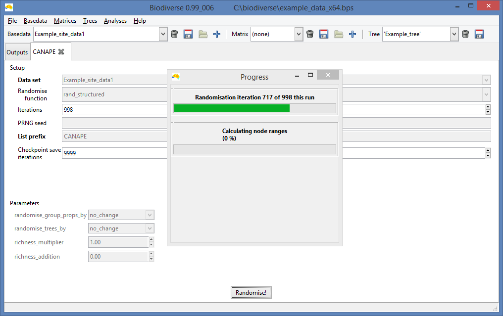Unsurprisingly, the progress bar displays how progress has been made.

Step 4.  View the randomisation results 

This is another case of "the images are in the previous blog post".  Look for step 2 in http://biodiverse-analysis-software.blogspot.com.au/2014/11/canape-categorical-analysis-of-palaeo.html  (but note that those images use a randomisation name of Rand1 instead of CANAPE).

Step 5.  Export the results 

Exporting the results in Biodiverse version 0.99_005 and later can be done while viewing the spatial output (see this previous blog post), or from the outputs tab.  In earlier versions exporting can only be done from the outputs tab. 

The screenshot below shows the export options.  If you are using the Biodiverse pipeline then you need to export to delimited text format files.  If you are going to hand roll your classification then use whichever format is appropriate. 

Choose the export option most appropriate to your needs. 

Export the SPATIAL_RESULTS list.  This contains all the PE and RPE results.  This image is for the Delimited text method.  Some options will differ for other export methods. 

Export the randomisation results. 

The delimited text exports can be viewed in a spreadsheet program or imported into a stats package such as R. 

The results are in two tables (one for the spatial analyses, one for the randomisation results) so might need to be linked.  Use the Element field in each table for this, as it is the unique identifier for each group (in Biodiverse a group is jut a special type of element, as is a label).  The Axis_0 and Axis_1 fields are the coordinates of the cell centroids.  There can be any number of axis columns in a basedata, but in this case we have only two.  Remember that the randomisation naming scheme is explained here. 

If you export to one of the raster formats (except the ER-Mapper format) then you will have one raster per list item, so one for PE_WE_P, one for RPE_NULL2, etc.  The ER-Mapper format packs all of one list into one multiband raster, with one band per list item.

Step 6.  Classify the data 

The next step is to classify the data into neo, palaeo and mixed-endemism. Blow-by-blow details of that will be left to another blog post, as this one is getting pretty long.  More of the pipeline also needs to be shaken out so it works with other data sets before I can write about that.

If you want to go ahead and do it yourself then it is not particularly complex.  Details of the classification system are given in the previous blog post.   Look for Step 3.  Use the indices PE_WE_P, PHYLO_RPE_NULL2 and PHYLO_RPE2 for PE_orig, PE_alt and RPE, respectively.


Shawn Laffan 20-Nov-2014

For more details about Biodiverse, see http://purl.org/biodiverse

For the full list of changes in the 0.99 series (leading to version 1) see https://purl.org/biodiverse/wiki/ReleaseNotes

To see what else Biodiverse has been used for, see https://purl.org/biodiverse/wiki/PublicationsList


You can also join the Biodiverse-users mailing list at http://groups.google.com/group/Biodiverse-users