Biodiverse version 3.00 has now been released

Biodiverse version 3.00 has now been released


Versions for Windows, Mac and Linux are available and can be downloaded from https://github.com/shawnlaffan/biodiverse/wiki/Downloads

Installation instructions are at https://github.com/shawnlaffan/biodiverse/wiki/Installation


Version 3.00 represents 44 issues closed across 350 source code commits.  187 files have been changed, with 13,623 insertions and 10,486 deletions.

Highlights of the changes since version 2.1 are at https://github.com/shawnlaffan/biodiverse/wiki/ReleaseNotes#version-300, and the related blog posts can be accessed via https://biodiverse-analysis-software.blogspot.com/search/label/Version3

A more detailed listing of the closed issues is at https://github.com/shawnlaffan/biodiverse/milestone/15?closed=1


The only change of note since the most recent development release (version 2.99_005) is to address issue #742.  The internal index used for matrices now uses the C locale for numeric values. Incorrect values could otherwise be returned in some locales where the comma is used as the radix character. Biodiverse now throws an exception when it encounters indexes with commas in the values, recommending that the matrix be rebuilt.



Shawn Laffan
03-September-2019


--------

For more details about Biodiverse, see http://shawnlaffan.github.io/biodiverse


To see what Biodiverse has been used for, see https://github.com/shawnlaffan/biodiverse/wiki/PublicationsList

You can also join the Biodiverse-users mailing list at http://groups.google.com/group/Biodiverse-users

Version 2.99_005 released, Version 3 is next

The final development release in the 2.99 series has now been released (2.99_005).

Barring any major issues, this will be the final development release before Version 3 is released.


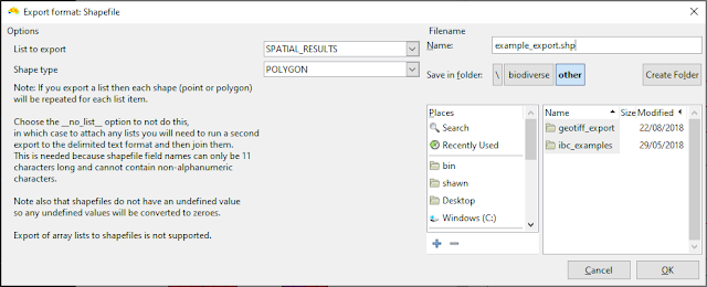
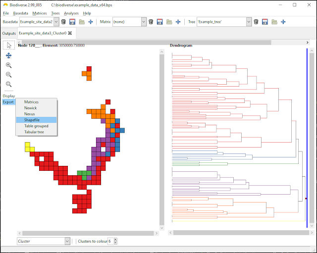
The main update in this version (from 2.99_004) is that the spatial patterns of cluster and region grower analysis outputs can now be exported to shapefile format, with each branch getting its own polygon or point features.  This means you can now use the polygon or point geometries for any branch in the tree for further analysis and/or display.  More details are in the blog post:  https://biodiverse-analysis-software.blogspot.com/2019/08/export-cluster-analyses-to-shapefiles.html


The more detailed summary of changes in the 2.99 series is at https://github.com/shawnlaffan/biodiverse/wiki/ReleaseNotes#version-299, and the related blog posts can be accessed via https://biodiverse-analysis-software.blogspot.com/search/label/Version3


This version can be downloaded from links on the downloads page at https://github.com/shawnlaffan/biodiverse/wiki/Downloads


Shawn Laffan
12-August-2019


--------

For more details about Biodiverse, see http://shawnlaffan.github.io/biodiverse


To see what Biodiverse has been used for, see https://github.com/shawnlaffan/biodiverse/wiki/PublicationsList

You can also join the Biodiverse-users mailing list at http://groups.google.com/group/Biodiverse-users

Export cluster analyses to shapefiles

In Version 3 of Biodiverse it is possible to export your cluster and region grower analyses to shapefile formats.

This makes it easier to use the regions in geospatial analyses, for example as conditions in spatial analyses in Biodiverse.  Perhaps the best example is that you can generate a regionalisation using one data set, and then assess its values for one or more other data sets.  See for example González-Orozco et al. (2013, 2014a and 2014b).

The option is available via the export menu for cluster and region grower analyses.  The options are all the usual ones, although that is not many in this case.

The option is chosen from the export menu for a cluster (or region grower) analysis.  

There are not that many choices, but Shape type can be exported as POLYGON or POINT geometries (shapes).  You can attach lists of results, or choose to only export the geometries themselves.

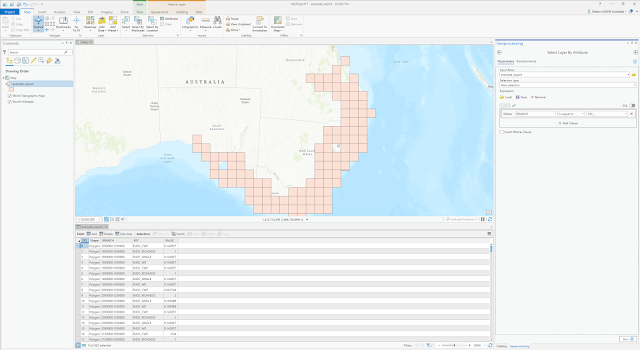
You might need to run a selection to highlight the branch you are interested in.  This example is branch 120___, which corresponds to the red cluster in the first screenshot above.  You might also choose to use a Definition Query (ArcGIS) or Layer Subset (QGIS) to filter out the geometries you are not interested in.  

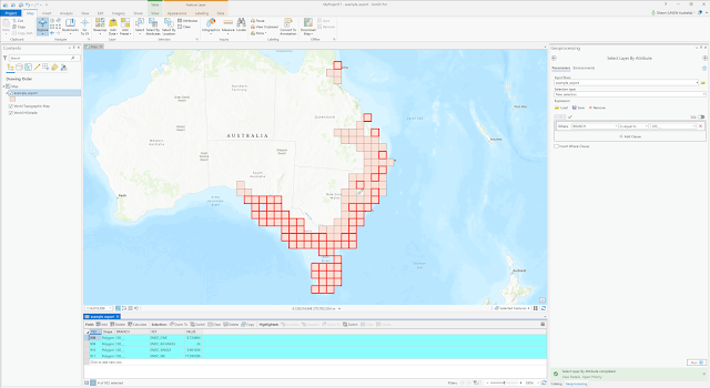
And here the component polygons that form the polygons for branch 120___ are highlighted in red.

There are three points to watch for.

1.  If you export a list with the data, then each polygon or point feature is repeated for each item in the list.  This is due to shapefile field names being limited to 11 characters, which is far too short for many of the list entries in Biodiverse.  (Support for the GeoPackage format is in the works to obviate this issue).

2.  The exported features (geometries) are multipolygon or multipoint.  This means that each geometry comprises one or more geometries, with each internal branch including all polygons of its terminal branches.  The internal boundaries between polygons are not dissolved, so you will see all the component polygons, but any GIS will support a dissolve operation.  If you are wondering what multipolygons and multipoints are, then Wikipedia has a decent explanation as part of the Well Known Text entry.

3.  Remember that Biodiverse knows nothing about coordinate systems and map projections (agnostic might be a better way of putting it).  You will need to define the coordinate system of the output file yourself using a GIS or other geospatial tool.



Shawn Laffan
12-August-2019

If you want to try this out before version 3 is released then the 2.99_005 development release can be accessed through the downloads page at https://github.com/shawnlaffan/biodiverse/wiki/Downloads


--------

For more details about Biodiverse, see http://shawnlaffan.github.io/biodiverse


To see what Biodiverse has been used for, see https://github.com/shawnlaffan/biodiverse/wiki/PublicationsList

You can also join the Biodiverse-users mailing list at http://groups.google.com/group/Biodiverse-users

Reproduce spatial plots with the same colours in GIS software

Biodiverse version 3 will allow users to export GeoTIFFs of the display colours for spatial outputs that have been displayed in the GUI.

The format used is RGBA (red, green, blue with a fourth Alpha channel for transparency).  This is a standard image format and is supported by many GIS packages.

This one is best demonstrated with pictures.  The GIS used is QGIS, but the general process is the same in ArcGIS.

The Acacia PD data displayed using a log scale with the default colour scheme. 

The RGB export is in the exports menu, with all the other exports.

The file selection is the usual process.  

And now in the GIS, the file is selected using the normal process.  Note that the file name is updated like the GeoTIFF exports, but with _rgb appended to the main part of the name. 

Biodiverse knows nothing about coordinate systems, so it is up to the user to choose the correct one for their data.  

The default display has all the colours, but the background is black.  To fix that you need to set the fourth band as the transparency layer.

As per the previous image caption, choose band 4 as the transparency layer.  The same general process is needed in ArcGIS (set the alpha channel to be band 4). 

And here is the data with some Open Street Map data in the background.  

And as a bonus, the RGB GeoTIFFs can be exported at the same time as a standard GeoTIFF export using the "Generate RGB Rasters" option.

As the tooltip states, the RGB files are only generated for indices that have been displayed, so you don't get huge numbers of exports if you have not displayed them.   

Shawn Laffan
20-May-2019

If you want to try this out before version 3 is released then the 2.99_004 (or later) development release can be accessed through the downloads page at https://github.com/shawnlaffan/biodiverse/wiki/Downloads

--------

For more details about Biodiverse, see http://shawnlaffan.github.io/biodiverse


To see what Biodiverse has been used for, see https://github.com/shawnlaffan/biodiverse/wiki/PublicationsList

You can also join the Biodiverse-users mailing list at http://groups.google.com/group/Biodiverse-users

Drop label and group axes

On occasion one might load a data set where the labels consist of several levels of the Linnean hierarchy, e.g. the name of a label will be made up of order, family, genus, species and subspecies.  Or you might have packed in extra information for debugging, or you have population ID included.

However, sometimes you want to simplify the records and use them at an different level.  For example, you might want to collapse your genus:species data to the genus level, or remove population and family details.

You might also have generated group names using geographic coordinates, plus additional details about time or region (see Stephenson  et al. 2015 and Laffan et al. 2013 for examples of those), but then want to remove the region or time axes.


One approach is to export the data (labels or groups) and then reimport them using only the axes you need, but this can be tedious as it involved several steps.  You could also use the rename interface with a remap table, but setting up the table can also be tedious.

From Version 3 it can be done directly within Biodiverse.

Some screenshots are probably the best way to explain it.  See captions for details.

The data in this case were used in Cassis et al. (2017) and consist of details downloaded from the Atlas of Living Australia .  Each label comprises the family, genus, scientific name and taxonomic level, joined using a colon (the standard join character used in Biodiverse).  This last column (axis) made it easier to remove records that were not at the species level, but is not needed for many analyses.  All these columns also make it hard to link the data to phylogenies.  (Note that they have no effect on indices like taxon endemism, rarity and richness, as those only need to work with unique identifiers).

Each label comprises four axes of information.  This can be useful, but not for everything.  

The process is done through one of the duplication options.  There is no undo, so it is safer to generate a new data set.

Unsurprisingly, the new basedata needs a name.

The system can work with either groups or labels.  If you need to trim axes from both then run it twice, once for groups and once for labels.  

Select which axes you wish to drop.  In this case only the scientific name will be retained.  Note that the axes are numbered from zero, which is common for many programming languages (but not for R).  

And here are the data with simplified labels.  Note that if, two or more labels collapse down to the same name then their sample counts are merged.  

And that's pretty much it.

The same process applies to groups so there are no screenshots provided for them.

Shawn Laffan
20-May-2019

If you want to try this out before version 3 is released then the 2.99_004 (or later) development release can be accessed through the downloads page at https://github.com/shawnlaffan/biodiverse/wiki/Downloads

--------

For more details about Biodiverse, see http://shawnlaffan.github.io/biodiverse


To see what Biodiverse has been used for, see https://github.com/shawnlaffan/biodiverse/wiki/PublicationsList


You can also join the Biodiverse-users mailing list at http://groups.google.com/group/Biodiverse-users

Unicode file names on Windows

Biodiverse can now handle unicode file names on Windows.

Previously if you had a file with a name like "mexaves 5 años mex.csv", "Havlærskilpadde.shp", "Grönfläckig padda.tif", or "Démonská kachna zkázy.xlsx" then it would fail to import.  This can be a considerable irritation if working on non-English locales.

The underlying details of why are better described elsewhere, but basically the file name passed by the GUI did not match the encoding scheme when the underlying Perl code went looking for it.

Thanks to the Win32::LongPath library we can work around this and use the full windows file name.

There are no screenshots for this post, but the implementation details can be seen here for those who are interested.

This also needs to be tested using CJK (Chinese, Japanese, Korean) characters.  Please report issues if any are found.

Shawn Laffan
20-May-2019

If you want to try this out before version 3 is released then the 2.99_004 (or later) development release can be accessed through the downloads page at https://github.com/shawnlaffan/biodiverse/wiki/Downloads

--------

For more details about Biodiverse, see http://shawnlaffan.github.io/biodiverse


To see what Biodiverse has been used for, see https://github.com/shawnlaffan/biodiverse/wiki/PublicationsList


You can also join the Biodiverse-users mailing list at http://groups.google.com/group/Biodiverse-users

Reduce the spatial resolution of your data

A longstanding wish-list item for Biodiverse is the ability to decrease the resolution of the cells (groups).  For example, you might have imported your data at a 50 km resolution but want to see what happens to the analysis results when the data are aggregated to 100 km.

This has just been implemented for version 3.  If you are impatient then you can try it in the 2.99_003 development release.  The download link is at the end of this post (and please provide feedback if you do try it).

Some screenshots will probably help explain things.  A few more details follow them.

The original data (100,000 units on a side) with some lines from a shapefile overlaid. 

The interface is accessed through the BaseData menu, and generates a new BaseData object

The interface allows control over the new name, the new resolution and the new origin.

In this example, the new cells will be 200,000 units on each side, with the cells aligning with an origin coordinate at (100,000, 100,000).  For these data it means that, if the cells span the coordinate (0,0) then it will be the centre of a cell.

And the new data with the reduced resolutions (200,000 units on a side), again with the lines so they can be cross-referenced with the original data.  Note how the sample counts for each label are the same, but the variety scores (number of groups each label is found in) are now smaller.    

There is nothing stopping rectangular groups, except perhaps a cultural preference for square cells.  

A few extra details:

The cell sizes can only ever be increments of the current cell sizes.  The data used in Biodiverse are commonly observations that have been aggregated to the groups (cells), and the original ditribution are not kept.  There is no good way of disaggregating the data to restore the original distributions.  This means you can aggregate to coarser units, but not go the other way.

The origins are also increments of the cell sizes, for the same reason.

The GUI will snap any values to increments of the cell size if users try to enter different values.

Text axes cannot be aggregated (although it could be done if there were a need and a good way of doing so).

Axes with zero cellsizes, e.g. where data are used as points, can be aggregated to any coarser resolution.  The system generates a default for each axis using the extent of that axis divided by 20 (so it will result in 20 cells along each axis by default).


Shawn Laffan
06-April-2019

If you want to try this out before version 3 is released then the 2.99_003 release can be accessed through the downloads page at https://github.com/shawnlaffan/biodiverse/wiki/Downloads

--------

For more details about Biodiverse, see http://shawnlaffan.github.io/biodiverse


To see what Biodiverse has been used for, see https://github.com/shawnlaffan/biodiverse/wiki/PublicationsList


You can also join the Biodiverse-users mailing list at http://groups.google.com/group/Biodiverse-users or follow the google plus page:  https://plus.google.com/+BiodiverseSoftware

Publications using Biodiverse in 2018

We are well into 2019, so here is a list of publications that used Biodiverse in 2018. 

If you want to see the full list (100 at the time of writing), then go to https://github.com/shawnlaffan/biodiverse/wiki/PublicationsList 

For more details about Biodiverse, see http://shawnlaffan.github.io/biodiverse/ 

Shawn Laffan

02-Apr-2019

Bloomfield, N.J., Knerr, N. and Encinas-Viso, F. (2018) A comparison of network and clustering methods to detect biogeographical regions. Ecography, 41, 1-10.

Carta, A., Pierini, B., Roma-Marzio, F., Bedini, G. and Peruzzi, L. (2018) Phylogenetic measures of biodiversity uncover pteridophyte centres of diversity and hotspots in Tuscany. Plant Biosystems, 152, 831-839.

Dalrymple, R.L., Kemp, D.J., Laffan, S.W., White, T.E., Flores-Moreno, H., Hemmings, F.A., Hitchcock, T.D., & Moles, A.T. (2018) Abiotic and biotic predictors of macroecological patterns in bird and butterfly coloration. Ecological Monographs, 88, 204-224.

Di Virgilio, G., Wardell-Johnson, G.W., Robinson, T.P., Temple-Smith, D., Hesforde, J. (2018) Characterising fine-scale variation in plant species richness and endemism across topographically complex, semi-arid landscapes. Journal of Arid Environments, 156, 59-68.

Elliott, M.J., Knerr, N.J. and Schmidt-Lebuhn, A.N. (2018) Choice between phylogram and chronogram can have a dramatic impact on the location of phylogenetic diversity hotspots. Journal of Biogeography, 45, 2190-2201.

Guedes, T.B., Sawaya, R.J., Zizka, A., Laffan, S.W., Faurby, S., Pyron, A., Bérnils, R.S., Jansen, M., Passos, P., Prudente, A.L.C., Cisneros-Heredia, D.F., Braz, H.B., Nogueira, C.d.C., & Antonelli, A. (2018) Patterns, biases and prospects in the distribution and diversity of Neotropical snakes. Global Ecology and Biogeography, 27, 14-21.

Laffan, S.W. (2018). Phylogeny-based measurements at global and regional scales. In R. Scherson & D. Faith (Eds.), Phylogenetic Diversity: Applications and Challenges in Biodiversity Science (pp. 111-129): Springer.

Link-Pérez, M.A. and Laffan, S.W. (2018) Fern and lycophyte diversity in the Pacific Northwest: Patterns and predictors. Journal of Systematics and Evolution, 56, 498-522.

López-Aguirre, C., Archer, M., Hand, S.J. and Laffan, S.W. (2018) Phylogenetic diversity, types of endemism and the evolutionary history of New World bats. Ecography, 41, 1955-1966.

Miu, I.V., Chisamera, G.B., Popescu, V.D., Iosif R., Nita, A., Manolache, S., Gavril, V.D., Cobzaru, I. and Rozylowicz, L. (2018) Conservation priorities for terrestrial mammals in Dobrogea Region, Romania. ZooKeys, 792, 133-158.

Montaño-Arias, G., Luna-Vega, I., Morrone, J.J., Espinosa, D. (2018) Biogeographical identity of the Mesoamerican dominion with emphasis on seasonally dry tropical forests. Phytotaxa, 376, 277-290.

Orsenigo, S. et al. (2018) Red Listing plants under full national responsibility: Extinction risk and threats in the vascular flora endemic to Italy. Biological Conservation, 224, 213-222.

Sosa, V., De-Nova, J.A. and Vásquez-Cruz, M. (2018) Evolutionary history of the flora of Mexico: Dry forests cradles and museums of endemism. Journal of Systematics and Evolution, 56, 523-536.

Spalink, D., Pender, J., Escudero, M., Hipp, A.L., Roalson, E.H., Starr, J.R., Waterway, M.J., Bohs, L. and Sytsma, K.J. (2018) The spatial structure of phylogenetic and functional diversity in the United States and Canada: An example using the sedge family (Cyperaceae). Journal of Systematics and Evolution, 56, 449-465.

Spalink, D. et al. (2018) Spatial phylogenetics reveals evolutionary constraints on the assembly of a large regional flora. American Journal of Botany, 105, 1938-1950.

Yap, J-YS., Rossetto, M., Costion, C., et al. (2018) Filters of floristic exchange: How traits and climate shape the rain forest invasion of Sahul from Sunda. Journal of Biogeography, 25, 838-847.

Zhang, H., Bonser, S. P., Chen, S.-C., Hitchcock, T. and Moles, A. T. (2018) Is the proportion of clonal species higher at higher latitudes in Australia? Austral Ecology, 43, 69-75.

Using the Run Exclusions dialogue

One of the processes users are often interested in is filtering their data after they have been imported.  This is often simpler than filtering a large  table of input data into multiple versions for different different purposes, especially if the input file is something like a 10 GB CSV file.


In Biodiverse this can be done using the Run Exclusions dialogue, accessed via the Basedata menu.

The main principle of this dialogue is to allow the user to select some set of properties, of either labels or groups, and then remove them from the basedata.  A simple example might be to remove all groups containing five or fewer labels, or labels with ranges exceeding some threshold.  More complex queries can also be specified using text matching (labels) or spatial conditions (for groups).

One can also delete labels using the selection menu in the View Labels tab (see this previous post), but this does not apply to groups (unless you transpose the basedata so you can treat the groups as labels, and then transpose them back).

An important point to note is that the Run Exclusions dialogue does not trigger updates in any open View Labels tabs.  If you delete labels or groups from a basedata then you will need to close and re-open any View Labels tabs for that basedata to see the changes.

It is also worth noting that the aggregation of labels to groups is a one way process.  The original input records cannot be recovered from a basedata object unless a cell size of zero is used (for numeric axis data) or there is only one record per text axis (when text axes are used).  It is impractical to store the 10 GB data from the example at the top.


The rest of this blog is just a set of examples.  The data are the example data provided with Biodiverse.   There are also details in the help system at https://github.com/shawnlaffan/biodiverse/wiki/SampleSession#excluding-data

The Exclusions dialogue is accessed through the Basedata menu.  Exclusions will apply to the currently selected Basedata object.  

View Labels tab showing the original distribution of data.  

This example uses a definition query to delete all groups whose centroid falls inside polygons where the state field has a value of 'Tas'.   

The system gives feedback about how much was deleted.  

Note the removal of most cells in Tasmania.  The reason not all cells are removed is that the centroid of some groups falls outside the polygon.  An overlap condition will be added one day, but until then the shapefile needs to be modified to catch these cases.

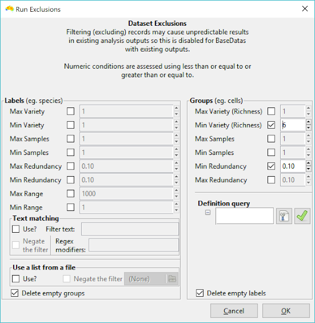
This example will remove all groups with fewer than 6 species, or where the sample redundancy score is less than 0.1.

The feedback (based on a fresh copy of the basedata)

Not much is left in this case...

This (highly contrived) contrived regular expression will delete any label ending in sp followed by any digit and ending in 2.  It will delete Genus:sp12, Genus:sp22 up to Genus:sp92, but not labels like Genus:sp2, Genus:sp83, Genus:sp222.  (Ignore the cursor between the 2 and the $)

And the feedback.  Only two labels are deleted, as the only matching labels in this basedata are Genus:sp12 and Genus:sp22.

That's about it, really.  If you have questions then they can be posted to the Biodiverse user group, or to the google plus page (until Google shuts that service down).

Shawn Laffan
28-Feb-2019


--------

For more details about Biodiverse, see http://shawnlaffan.github.io/biodiverse


To see what Biodiverse has been used for, see https://github.com/shawnlaffan/biodiverse/wiki/PublicationsList


You can also join the Biodiverse-users mailing list at http://groups.google.com/group/Biodiverse-users or follow the google plus page:  https://plus.google.com/+BiodiverseSoftware