Biodiverse is probably best known for its ability to link phylogenies to spatial data, but that's only a subset of what it can do. It can also attach properties to each label, for example species traits like average height, seed type, locomotion method or growth form. This has been available for several versions.
Examples using label properties include colour across birds, butterflies and flowers (Dalrymple et al.
2015,
2018), plant longevity (Zhang et al.
2018), fleshiness (Chen et al.
2017), spinescence (Tindall et al.
2017) and fruit fleshiness (Rossetto et al.
2015).
The analysis of group property data has also proven useful, for example when summarising environmental conditions in bioregionalisation analyses, example González-Orozco et al. (
2013,
2014a,
2014b). In these cases one assigns a value to each group (cell) to describe, for example, the mean grain size across its area. At the moment the matching system uses exact matches on element (cell) names, so these need to be set up for the data to be correctly attached. This can be done by importing the environmental data into Biodiverse, one layer at a time, at the same resolution and origin as the species data, and then exporting to delimited text. The exported file will then have element names that match exactly when imported into Biodiverse as group properties.
And as a nice example that one does not need to work only with species and cells, the data in Stephenson et al. (
2015) represent a spatio-temporal data set of larval herring size classes. These are first analysed on a per-year basis across all locations, then on a per-location basis across time periods using group properties. See the
supplementary material of that article for more detailed steps.
So how does one analyse such data using Biodiverse? The overview is simple - one attaches the data to a BaseData object, then one analyses it. Examples are below, followed by some other considerations like deletion, but a few concepts need to be given first.
- In Biodiverse, trait data are called "properties". This is a deliberately generic term, as there is no reason why one could not analyse non-biological phenomena using the system. (And we aim to be generic when developing Biodiverse, after all the the computer only sees numbers - it is the user who defines the analyses and interprets the results).
- If you are analysing trait data then you want to assign and analyse Label Property data. This is because one can also analyse Group Properties (see below).
- Both Labels and Groups are called Elements (also a more generic term), so the relevant calculations are under the "Element Properties" section of the calculation lists.
Attaching data
This is probably best demonstrated using images of the steps with captions.
If your label property data do not match exactly, then you can use the
remapping tools introduced in Version 2.
 |
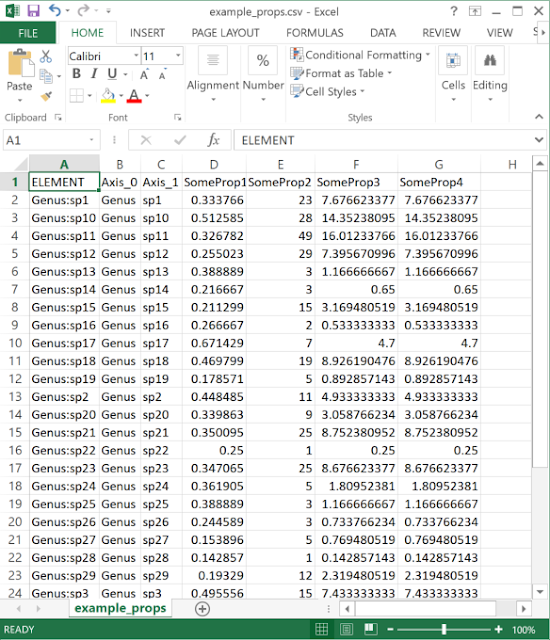
| The data need to be in a delimited text (e.g. CSV format) file. One column should match the element (label or group) name, while any number of others can be properties. |
 |
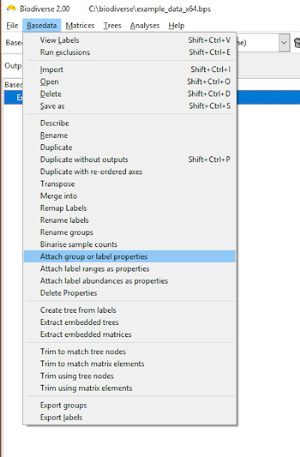
| The menu option is under the Basedata menu. |
 |
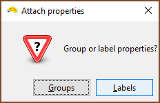
| One then chooses if the properties to be assigned are for groups or labels. In this example labels are selected. |
 |
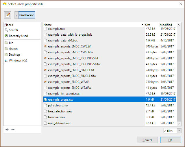
| The file selection is the usual process. |
 |
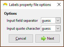
| Choose the field delimiter (usually a comma) and quote character. |
 |
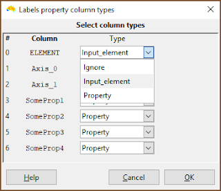
| This is the important bit. Make sure the column with the element names in it is specified as Input_element. (It does not need to be called ELEMENT). |
 |
| Make sure that any column containing property data are specified as Property. Any column with Ignore is ignored by the system. |
 |
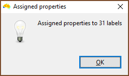
| Once run, you are told how many labels or groups had properties assigned. If there were fewer than you would expect then check the column you specified as Input_element contains matching items. Be careful with quotes, and remember that spreadsheet programs can do odd things with your data when they import them, so use a text editor to be certain. |
 |
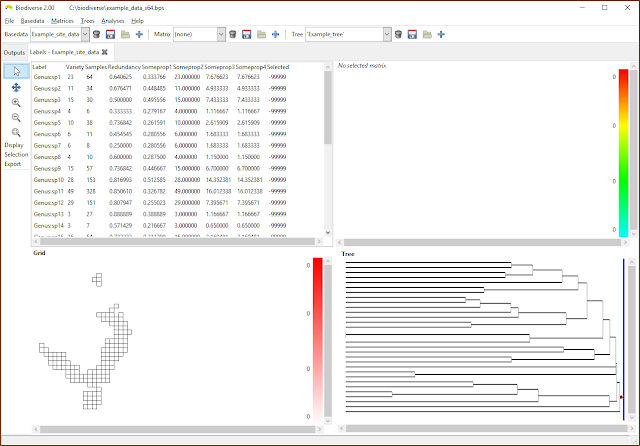
| Any label properties will now be shown as additional columns in the list in the View Labels tab. |
Analysing properties
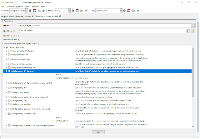
Analysis of properties follows the usual process. The example below is for a spatial analysis, but similar selections apply in the cluster and region grower analyses.
The most important point to understand is that the results are stored as lists, and not as single scalar indices. This make it easier to organise the results across arbitrarily named properties.
 |
| The property calculations are under the Element Properties groups in the calculations lists. |
 |
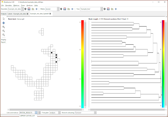
| Select the list containing the desired indices. If only property calculations have been chosen then the SPATIAL_RESULTS list will be empty. (Note that the menu has been cropped by the screenshot in this case). |
 |
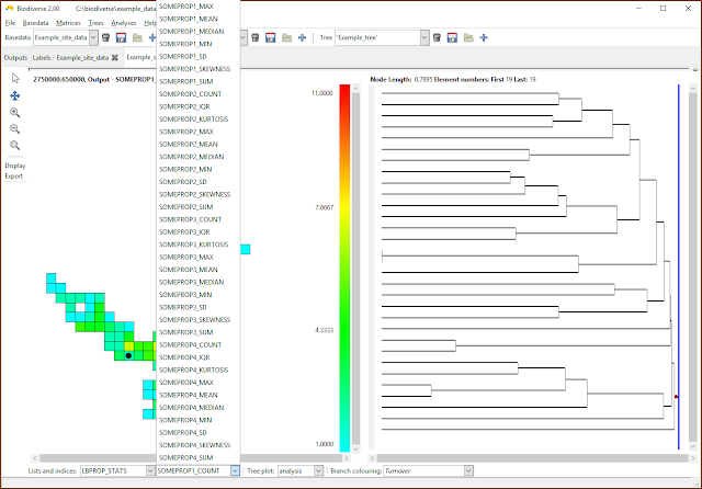
| Now choose the index to be displayed. Many of the calculations create indices in the lists that are some combination of the property name as a prefix, hence the repetition of suffixes in this example. |
 |
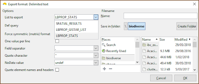
| Be sure to select the desired list when exporting. |
Attaching ranges and abundances
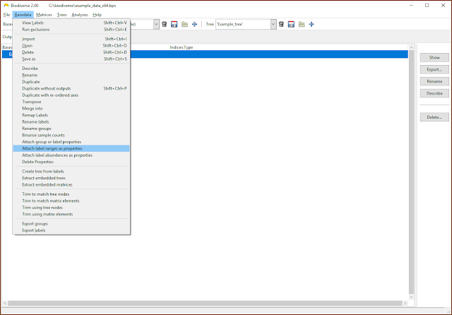
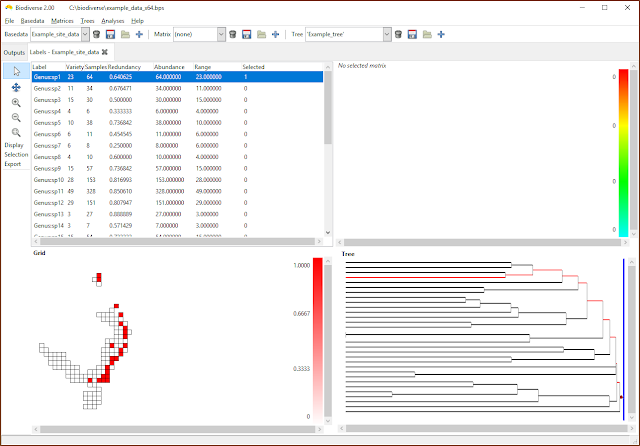
One can also attach the label ranges and abundances as label properties, as per the next two screenshots. Be aware, though, that these are not dynamically updated. If you add or delete groups then these will need to be updated (unless, of course, you want the old values).
 |
| Label ranges and abundances can be attached as properties |
 |
| Once attached, label ranges and properties are displayed and treated just like any other property. |
It's a bit of a kludge, but if you want to attach the cell richness and sample counts for groups, then you can transpose the basedata to create a new basedata object, so the old groups are labels and the old labels are now groups. Then attach the label ranges and abundances (remember the labels in the new object are the groups in the previous object) and transpose the data again to get back to the original structure. This process works because the way data are stored in Biodiverse can be treated as a matrix, where the rows are the groups and the columns are the labels (consistent with many other related implementations). The label ranges are the counts of the non-zero column entries, and the group richness scores are the counts of the non-zero row entries. If one transposes the data then the column summations of the transposed data are on the old rows, and the same applies for the row summations.
Can I use categories directly?
Not yet.
An implementation detail is that the property data need to be numeric, so if you have nominal classes like "gravity" or "ballistic" for seed dispersal, then you need to code them as one column each, with a value of 1 for when the trait applies, and 0 if not. If there are unknown values then they can be left as blank and they will be ignored in the analyses. One day we will handle categorical data.
Can I delete some of the properties after importation?
Yes, and this has been possible since version 2 was released.
While the property import interface does not yet support column ranges (each column needs to be selected manually, which gets tedious...), one can still import more columns than are needed through inattention or because the process is automated in some way (or both).
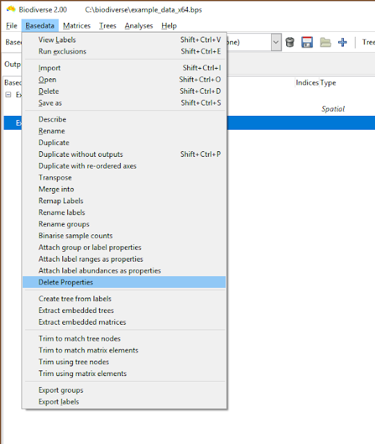
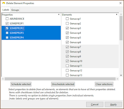
The deletion interface needs work, but is at least functional. There is one tab for label properties, and one for group properties. In either tab, select properties and schedule them to be deleted across all groups or labels, or choose labels and groups (elements) that will have all their property values cleared. Nothing is actually deleted until the Apply button is pressed, and entries can be deselected.
 |
| Property deletion is accessed via the Basedata menu |
 |
| The current interface needs work, but one can select rows and then schedule those entries for deletion. In this example, SOMEPROP1 and SOMEPROP2 will be removed from all groups, while labels Genus:sp3 to Genus:sp10 will have all their property values removed. |
It is also not possible to delete properties from a BaseData that contains outputs, even if those outputs do not use the properties. If there is a need to do so then please raise an issue using the
issue tracker. Until it is supported, you can use the
Basedata > Duplicate without outputs menu option to create a new BaseData with the same labels, groups and properties, but without any of the analysis outputs attached. Then delete the non-required properties.
Shawn Laffan
22-Aug-2018


