Biodiverse now calculates CANAPE for you

The CANAPE protocol is one of the analyses Biodiverse is most commonly used for (see examples amongst the list of publications using Biodiverse).  

The method, or protocol, was originally described in Mishler et al. (2014) and is conceptually simple.  Run an analysis that includes phylogenetic endemism and relative phylogenetic endemism, run those through a randomisation, and then categorise the results based on the significance score of the indices.  This process is described in more detail in previous posts here and here.  

The main issue with the approach to date is that the CANAPE classes are determined outside of Biodiverse using systems like a GIS, R code or a spreadsheet.  So while the process is conceptually simple, the actual implementation can all get a bit complex. Many users are not entirely sure which indices to pass through their functions, or even which lists to extract them from.  

As of Version 4 Biodiverse now calculates it for you.  This occurs automatically whenever an analysis has included the Phylogenetic Endemism and Relative Phylogenetic Endemism type 2 calculations.   (If you want it sooner than version 4 then it is in the development release 3.99_005, which was current at the time of writing.  See the downloads page for links).

Biodiverse now calculates the CANAPE scores when the requisite indices have been calculated, and a randomisation has been run.  Like many of the posts on this blog, this example uses the Acacia data set from Mishler et al. (2014).

How does Biodiverse store the results? 

The results are stored in a new list where the name is the randomisation output used followed by ">>CANAPE>>".  So for a randomisation called "rand" you would see "rand>>CANAPE>>".  The use of angle brackets might look a bit strange at first but makes the naming consistent with the other randomisation lists and simplifies the underlying code.

The CANAPE classes are stored in an index called CANAPE_CODE, with a numeric code indicating which of the categories a cell falls in.  Currently this code is 0 for not significant, 1 for neo-endemism, 2 for palaeo-endemism and 3 for mixed endemism.

Biodiverse also provides individual indices for neo, palaeo and mixed in the event a user only wants to see which cells are are in a specific class.  For example one might want to run a cluster analysis using only neo-endemism cells following the process described here.  

 

The same data as above but highlighting Palaeo-endemism cells in red.  All other cells containing data are in blue.  

Visualisation

A big advantage of generating CANAPE results within Biodiverse is that users can now explore the results using the functionality Biodiverse provides.  As an example, the next screen shot shows an exploration of the contribution of each clade on the tree in relation to the analysis groups (cells) (see more details about that process here and here).  

Each tree branch is coloured by the relative contribution of the clade subtending it to the PE score in the cell being hovered over (black dot in south-western WA).  This allows an understanding of which clade is driving the PE scores, and thus CANAPE, in a cell.  The visualisation process is explained in more detail here.  

Displaying the results in other systems

If you then want to use the plots as part of a map then they can be exported to an RGB Geotiff.  Details of how to do this are in another post but the next two screenshots show the start and end.  

What about a different colour scheme?

The colour scheme used is from Mishler et al. (2014) where neo is red (new is hot), palaeo is blue (old is cold) and purple is between blue and red on a colour wheel.  

If you prefer a different colour scheme then you can export the data as you normally would, for example as CSV files or as non-RGB geotiffs, and recreate the plot to your own tastes.  

Changing the colours within Biodiverse would be very useful and contributions are always welcome.

What about the Super class?  

The system does not currently generate the Super class.  It can be added if there is demand.  (Edit: It was added for Biodiverse Version 5).

Do I have to run a new randomisation analysis to see the CANAPE list?  

The CANAPE lists are generated at the end of any sequence of randomisations.  If you already have a randomisation analysis then they can be created by running one additional iteration.  

If you are concerned that your analysis is already at 999 iterations then all you lose is a bit of numeric neatness as there are now 1001 realisations in total instead of 1000 (one original plus all the random ones).  This is unlikely to make any meaningful difference once that many iterations have been run.

--------

Shawn Laffan

25-Oct-2022

For more details about Biodiverse, see http://shawnlaffan.github.io/biodiverse/  

To see what else Biodiverse has been used for, see https://github.com/shawnlaffan/biodiverse/wiki/PublicationsList 

You can also join the Biodiverse-users mailing list at https://groups.google.com/group/Biodiverse-users or start a discussion at https://github.com/shawnlaffan/biodiverse/discussions 

Visualise spatial analysis results on the tree

Many of the indices in Biodiverse allow users to see what the relative contribution of branches on the tree are to one or more indices.  For example, one can see what the weighted branch lengths are in a phylogenetic endemism analysis, or see what the relative loss of phylogenetic diversity would be if a branch was lost from a sample.

Previously the only way to inspect these was to use a popup window by control-clicking on a cell.  This is useful, but rapidly becomes difficult when there are many cells to explore.

In version 2 of Biodiverse, users can now visualise these values on the tree as the mouse is hovered over cells.

This builds on the turnover displays that were added a while ago.

Rather than a long blog post, it is probably best to simply show a video.  In this example, a set of indices are calculated for the Acacia data set described in several publications (see the full list here and search for Acacia).

Note how the display is log scaled by default, but linear scaling can be used if preferred.  The default colour scheme uses the rainbow-ish default, as in the map display, but other schemes can also be used.  Users can also hide the legend if it gets in the way.

Shawn Laffan

19-Aug-2017

For more details about Biodiverse, see http://purl.org/biodiverse 

For the full list of changes in the 1.99 series (leading to version 2) see https://purl.org/biodiverse/wiki/ReleaseNotes (for all issues addressed or being targeted to fix for version 2, see https://github.com/shawnlaffan/biodiverse/milestone/4 ).

To see what else Biodiverse has been used for, see https://purl.org/biodiverse/wiki/PublicationsList

You can also join the Biodiverse-users mailing list at http://groups.google.com/group/Biodiverse-users

Biodiverse now categorises your randomisation results

[[ 2016-08-30:  This post has been superseded - the categorisation was not sufficiently clear.  See this followup post for how the system works now ]]


One of the issues users face with the randomisations in Biodiverse is what to do with them once they have been run.

One key point is that the results are stored on the other analysis objects themselves, as extra indices and lists.  The index names themselves are a bit cryptic, but are consistent, and there is a description of what they mean here:  https://purl.org/biodiverse/wiki/AnalysisTypes#where-do-the-randomisation-results-go-and-what-do-they-mean

Even then, it can be difficult working out which of your groups have index scores that are significantly different from the randomisation.  This is because the data are plotted as a continuum (which in turn is because it uses the same plotting process as the original index scores).  The first image below is an example of this plotting.

One can easily  export the data and work with them in a GIS or stats package, but any tied values need to be factored in for lower tail tests, for example as used in the CANAPE process.

With the next version of Biodiverse this categorisation will become a little easier.  Biodiverse will automatically categorise your randomisation results into significance levels, putting the results into new lists on the objects that can be displayed and exported in the same way as any other data.

As an example, imagine you have run a randomisation analysis for a BaseData containing a spatial analysis in which you calculated phylogenetic endemism.  Assume that the randomisation's name is rr (not a good name, but it's convenient to type here), so the spatial analysis will now have three lists you can plot.  The first two are the same as ever:  SPATIAL_RESULTS contains the observed results for each group (cell), and rr>>SPATIAL_RESULTS contains indices to track the randomisations for each index in SPATIAL_RESULTS.  For example, for PE_WE there will be C_PE_WE, Q_PE_WE, T_PE_WE and P_PE_WE collating, respectively, the number of times observed PE_WE was higher than that generated using the randomised data, the number of time observed PE_WE was compared against the scores from the randomised data, the number of times the observed and random scores were tied, and the proportion of iterations that the observed score was higher than the random scores (P_PE_WE = C_WE_PE / Q_PE_WE).

The new list is rr>>sig>>SPATIAL_RESULTS.  This contains a set of categorisations for one and two tailed tests for each index found in SPATIAL_RESULTS.  The lower tail tests take into account any ties in the comparisons.  An example plot is in the second image below.

For the PE_WE example, one has SIG_1TAIL_PE_WE and SIG_2TAIL_PE_WE.  SIG_1TAIL_PE_WE is a one-tailed test for higher or lower than expected.  It has a value of 0.01 if it is significantly high at alpha=0.01, 0.05 if high for alpha=0.05, -0.01 if it is significantly low at alpha=0.01, and -0.05 for low at alpha=0.05.  If it is not significant then it has a null (undefined) value.

SIG_2TAIL_PE_WE has the same numbers, but for a two tailed test.  Values of -0.05 and 0.05 are low or high for a two tailed alpha=0.05, i.e. the observed scores are in the outer 5% of the distribution of random scores (<2.5% or >97.5%, respectively), while those with -0.01 or 0.01 are in the outer 1% and significant at alpha=0.01.

The upper and lower one-tailed tests have been combined into the same list to reduce the number of indices and lists generated, and thus use less memory and disk space (an index cannot be both significantly high and low so there is no overlap).  If you are interested in a one tailed test for high values then ignore the low values, and vice-versa.  The values can be easily separated after exporting the results.

Currently the results are plotted in the same manner as any data, but there are plans to allow users to overlay the randomisation significance results over the top of the observed results, for example by masking our any non-significant scores.

The current system plots all scores, regardless of whether they pass a threshold or not.  This is useful, but is difficult to interpret when looking for significance against the randomisation.

The new categorisation filters out any score that is not significant at an alpha level of either 0.05 or 0.01 (here the one-tailed results are plotted, so negative values are significantly low).  The plotting could be improved, but it will work well enough now for exploration - proper maps can also be made using a GIS or stats package.  

This is a new implementation, so any feedback about usability would be very useful.  

Shawn Laffan

06-Aug-2016

For more details about Biodiverse, see http://purl.org/biodiverse 

For the full list of changes in the 1.99 series (leading to version 2) see https://purl.org/biodiverse/wiki/ReleaseNotes 

To see what else Biodiverse has been used for, see https://purl.org/biodiverse/wiki/PublicationsList

You can also join the Biodiverse-users mailing list at http://groups.google.com/group/Biodiverse-users 

More CANAPE - how to restrict your cluster analysis to groups with significant endemism

Two previous posts described more of the background to the CANAPE analysis and how to do it yourself.

[[  2017-08-10 UPDATE - the second part of the condition used an incorrect index name, so the clustering only applied to the palaeo and some of the mixed cells.  This has been corrected in the post.  ]]


What was not covered in those posts was the final step in the Mishler et al. (2014) paper in which the cells classified as palaeo- neo- or mixed-endemism under the CANAPE scheme were clustered to identify groupings with shared branches from the tree.

The aim of this post is to fill that gap.


The way it is done is conceptually simple.  We just need to constrain the cluster analysis to only use cells that are identified as having significant phylogenetic endemism.  The way it is done takes just a few steps, and a bit of typing.


Analyses in Biodiverse can be constrained to work only on a subset of groups (cells) using a definition query (the same as a "where clause" used in database queries).  The way it is currently done is a little more involved than is ideal, largely due to the amount of typing needed, but is not too complex to get working.  (One day we will develop a spatial conditions builder interface to make spatial conditions easier).

So, imagine you have run a spatial analysis called "phylo_end" in which you have told the system to calculate the indices under the  Phylogenetic Endemism and Relative Phylogenetic Endemism, type 2 calculations.  You then ran 999 iterations of a randomisation called CANAPE to assess how often the observed index values were higher than random.  The spatial results object now has an additional list called CANAPE>>SPATIAL_RESULTS which contains the counts of how often the observed value was higher than the randomised values, how many iterations were applied for each index, how many ties there were, and the proportion that were higher than random.  (See the help for more details about the naming scheme).

An example of the setup for the randomisation.

The randomisations have been completed so now the spatial analysis has an output list called CANAPE>>SPATIAL_RESULTS.  This list contains indices that summarise how often the observed values were higher than (or tied with) those calculated using the randomised data.

The next step is to start a new cluster analysis and set our definition query.  The selected basedata has a randomisation output, so you will be warned about possible issues with synchronisation.  This is only a potential problem if you run more iterations of the randomisation, which is not the case here so you can safely ignore the warning.

You will see this warning when you open a new cluster analysis, but can ignore it in this case.  

Set the Metric to be PHYLO_JACCARD (or whatever metric you like - it is your analysis after all) and enter the text below in the Definition Query box (you will need to expand it to enter text).  If your output and randomisation names differ then edit the text as appropriate.

sp_get_spatial_output_list_value (
    output => 'phylo_end', 
    list   => 'CANAPE>>SPATIAL_RESULTS', 
    index  => 'P_PE_WE'
) > 0.95
|| 
sp_get_spatial_output_list_value (
    output => 'phylo_end', 
    list   => 'CANAPE>>SPATIAL_RESULTS', 
    index  => 'P_PHYLO_RPE_NULL2'
) > 0.95



What this does is use the sp_get_spatial_output_list_value() subroutine to access the randomisation indices.  If either of the PE scores for a group using the observed or alternate trees are higher than the randomisations for 95% of iterations (these are the P_PE_WE and P_RPE_NULL2 indices) then that group will pass the test. Only those groups (cells) that pass the test will be considered for the cluster analysis.

Example of the cluster analysis setup, with a definition query specified.  Only those groups (cells) that pass the test will be used in the cluster analysis.
(The text in the image is different from the main text only in whitespace and formatting.  The code is the same).    

Once the analysis is run it will look something like the image below.

Completed cluster analysis.  Cells that failed the definition query were not considered for clustering and are plotted in grey.  

And there it is, a cluster analysis of the CANAPE regions to identify which ones have similar sets of branches from the tree.

Of course, definitions queries are extremely versatile and can be used for all sorts of applications.  You might, for example, want to cluster within a region defined by a shapefile but consider geographic ranges from across a broader study region.

It is also worth noting that spatial analyses can use definition queries, but they affect the analysis differently.  Calculations will only be completed for groups that pass the definition query, but those groups can have neighbours that fail the definition query.  This allows one to more easily analyse data with larger window sizes but with a guard area (data on the edges of the analysis region which, if not considered, could cause biased results).


Shawn Laffan, 19-Apr-2016


For more details about Biodiverse, see http://purl.org/biodiverse

To see what else Biodiverse has been used for, see https://purl.org/biodiverse/wiki/PublicationsList

You can also join the Biodiverse-users mailing list at http://groups.google.com/group/Biodiverse-users

Do it yourself CANAPE

[[ Update 2022-10-25:  Biodiverse now calculates CANAPE for you, so steps 4-6 below are not needed to generate CANAPE maps and data.  See more details in this blog post. ]]

In the previous blog post I described some of methods behind the CANAPE (Categorical Analysis of Neo and Palaeo Endemism) method.

The purpose of this post is to give more details about how to run it with your own data.  You can also use the Biodiverse pipeline, but these instructions focus on how to do it using the Biodiverse GUI (at least to the point of generating all the necessary data). 

These instructions assume you have already imported all your data, so both the species distribution data and the tree.  Instructions for how to do so are in the quick start guide.

The CANAPE analyses also need a version later than 0.19, which at the time of writing is the development version 0.99_005. [Update 2015-04-20 - version 1.0 has now been released http://purl.org/biodiverse/wiki/Downloads ]

Step 1.  View the data

This is a general step you should always do anyway, but open the View Labels tab so you can cross check the spatial data (the basedata object in Biodiverse parlance) and the tree.  This is accessed by the menu option Basedata->View Labels, the keyboard shortcut Shift-Control-V, or by double clicking on the basedata object in the outputs tab. 

As you hover over cells on the map (cells are called groups in Biodiverse) you should see paths on the tree being highlighted.  As you hover over branches on the tree you should see cells being highlighted.  If you click on cells or branches then species names (labels) in the list at the top left should be highlighted.

Hovering over a cell highlights any branches on the tree that are found in that cell. 

Hovering over a branch highlights the set of cells containing any of the named branches beneath it (usually just the terminals).  Clicking on the branch will also select the matching labels in the list at the top left, and colour all cells in the map based on how many of those labels are found in the associated group. 

If there is no highlighting then there is a mismatch between your tree and the basedata.  You will need to either rename the labels, for which there is an option in the basedata menu, or re-import the tree and specify a remap table when you do so.  Both approaches can use the same table, so it is up to you which data set should be the canonical source of names.  It does not matter which one is canonical for CANAPE, but for other analyses it can do.  It depends on what you want to do with the data.

Step 2.  Run the spatial analyses

The next step is to run the calculations for the observed data.  This uses a spatial analysis, and can be run using menu option Analyses->Spatial.  You should see something like the image below.  Make sure the tree you want to use is selected. 

The initial spatial analysis window with default spatial conditions. 

We now need to change the settings.  For this particular analysis we are only interested in each group (cell) in isolation, not collections of groups, so we need to delete the second spatial condition.

We also need to select the Phylogenetic Endemism calculation.  This can be accessed under the Phylogenetic Endemism category (or Phylogenetic Indices if you are using a version earlier than 0.99_005, but remember that CANAPE won't work on version 0.19 since it lacks the next set of calculations).  Then select the Relative Phylogenetic Endemism, type 2 calculation under the Phylogenetic Indices (relative) category.

Delete the second spatial condition and select the Phylogenetic Endemism calculation.

Also select the Relative Phylogenetic Endemism, type 2 calculation. 

When all is selected, hit the Go! button.  The example data set distributed with Biodiverse will take very little time to run.  The data set used in Mishler et al. (2014) takes approximately 5 seconds on a modern laptop.  (The code includes a number of optimisations such as caching of results for later re-use and binary searches where possible).

Step 2.  View the results

Now you get to bask in the glory of a set of results.

Screenshots of the example data are given in the previous blog post so won't be repeated here.  See the section "Step 1" at this URL:   http://biodiverse-analysis-software.blogspot.com.au/2014/11/canape-categorical-analysis-of-palaeo.html

It is time to stop basking and get back to work.

Step 3.  Run the randomisations

To assess which of the cells are candidates for palaeo- or neo-endemism we need to run a randomisation.  In this case we select the rand_structured option in Biodiverse, constraining the richness of each group (cell) to be equal across all randomisations.

CANAPE uses the rand_structured randomisation to ensure the richness of each cell is constant across all randomisation iterations/realisations. 

In the screen shot above you can see in the Setup section that we have chosen the rand_structured function for the randomisation.  We will run 999 iterations with all results being prefixed with "CANAPE".  See the Biodiverse help system for more details on the naming scheme.  The checkpoint save iterations is useful when one wishes to track a long running randomisation process to see if it has converged.  The basedata will be saved at any iteration ending in the value given will be saved, so a setting of 99 means iteration 99, 199, 299 etc will be saved.  It is probably not needed here, so can be set to 999.  [[EDIT 2020-Feb-19:  The checkpoints were used when we had crashes due to memory leaks.  These were fixed in version 0.18.  Unless you was to see how the system is progressing, the checkpoint save option can be set to -1 so it never happens.]]

The Parameters section allows us to control other options.  In this case we will leave the trees alone (randomise_trees_by equals no_change), so each analysis across the random iterations will use the original tree (for other analyses one might choose to randomise the tree but not the spatial data).  We have no group properties set so can also leave randomise_group_props_by as no_change.  A richness_multiplier of 1 and richness_addition of 0 means we will replicate the exact richness scores, as the formula used is a linear function (max_random_richness = observed_richness * richness_multiplier + richness_addition).


Now we hit the Go! button again.  This might take a while, depending on how large your data set is.  For the example data it is about 3 minutes on a modern laptop, but it can scale to hours for data sets of the size used in Mishler et al. (2014).

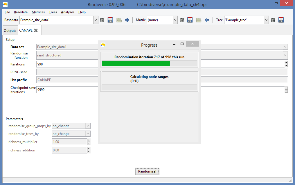
Unsurprisingly, the progress bar displays how progress has been made.

Step 4.  View the randomisation results 

This is another case of "the images are in the previous blog post".  Look for step 2 in http://biodiverse-analysis-software.blogspot.com.au/2014/11/canape-categorical-analysis-of-palaeo.html  (but note that those images use a randomisation name of Rand1 instead of CANAPE).

Step 5.  Export the results 

Exporting the results in Biodiverse version 0.99_005 and later can be done while viewing the spatial output (see this previous blog post), or from the outputs tab.  In earlier versions exporting can only be done from the outputs tab. 

The screenshot below shows the export options.  If you are using the Biodiverse pipeline then you need to export to delimited text format files.  If you are going to hand roll your classification then use whichever format is appropriate. 

Choose the export option most appropriate to your needs. 

Export the SPATIAL_RESULTS list.  This contains all the PE and RPE results.  This image is for the Delimited text method.  Some options will differ for other export methods. 

Export the randomisation results. 

The delimited text exports can be viewed in a spreadsheet program or imported into a stats package such as R. 

The results are in two tables (one for the spatial analyses, one for the randomisation results) so might need to be linked.  Use the Element field in each table for this, as it is the unique identifier for each group (in Biodiverse a group is jut a special type of element, as is a label).  The Axis_0 and Axis_1 fields are the coordinates of the cell centroids.  There can be any number of axis columns in a basedata, but in this case we have only two.  Remember that the randomisation naming scheme is explained here. 

If you export to one of the raster formats (except the ER-Mapper format) then you will have one raster per list item, so one for PE_WE_P, one for RPE_NULL2, etc.  The ER-Mapper format packs all of one list into one multiband raster, with one band per list item.

Step 6.  Classify the data 

The next step is to classify the data into neo, palaeo and mixed-endemism. Blow-by-blow details of that will be left to another blog post, as this one is getting pretty long.  More of the pipeline also needs to be shaken out so it works with other data sets before I can write about that.

If you want to go ahead and do it yourself then it is not particularly complex.  Details of the classification system are given in the previous blog post.   Look for Step 3.  Use the indices PE_WE_P, PHYLO_RPE_NULL2 and PHYLO_RPE2 for PE_orig, PE_alt and RPE, respectively.


Shawn Laffan 20-Nov-2014

For more details about Biodiverse, see http://purl.org/biodiverse

For the full list of changes in the 0.99 series (leading to version 1) see https://purl.org/biodiverse/wiki/ReleaseNotes

To see what else Biodiverse has been used for, see https://purl.org/biodiverse/wiki/PublicationsList


You can also join the Biodiverse-users mailing list at http://groups.google.com/group/Biodiverse-users

CANAPE - Categorical Analysis of Palaeo and Neo Endemism

[[ Update 2022-10-25:  Biodiverse now calculates CANAPE for you.  See more details in this blog post. ]]

The purpose of this blog is to explain in a bit more detail how the CANAPE method works.  This was prompted by some very useful questions from Stu Marsden.

The paper describing the CANAPE method (Mishler et al. 2014) is at http://dx.doi.org/10.1038/ncomms5473


The CANAPE method is a three step process.  In Step 1 a set of three primary indices as calculated for each region in the data set, in Step 2 a randomisation is run to identify regions with significant endemism.  In Step 3 these regions are classified into palaeo, neo, mixed or non-endemism.

Step 1.  Calculate the observed endemism 

The first step is to calculate a set of three observed endemism scores for each region in the data set:

1. Phylogenetic Endemism (PE) calculated using a user specified tree.  This will be called PE_orig below.  
2. PE calculated using an alternate tree.  This will be called PE_alt below.  
3. Relative Phylogenetic Endemism (RPE) which is calculated as the ratio of PE_orig to PE_alt. 

In this case each region is a single cell, but it could be any collection of cells for which one is interested in running the calculations.


The formula for PE for a region "i" is:




where is the set of branches found in region i, is the local range of branch (the number of cells in region i in which it is found), and is the global range of branch (calculated as the number of cells in which it is found across the whole data set).  Put in words, PE for a region is the sum of the branch lengths found in that region, but where each branch is weighted by the fraction of its geographic range that is found in that region.  It is worth noting that PE is basically is a range-weighted variant of PD (phylogenetic diversity), as the sum of PE scores across all cells will equal the PD for the set of branches found in those cells.

PE_orig and PE_alt are calculated in the same way, the difference is simply in the trees being used.  In Mishler et al. (2014) the alternate tree is one with the same topology as the original tree but where the non-zero branches are modified to be of equal length.  It should be noted that the per-branch range weighting is the same as for PE_orig, so each equalised branch receives the same range weighting as its counterpart in the original tree.

RPE for a region is simply the ratio of PE_orig and PE_alt for that region, so will be >1 when the original tree has longer range weighted branches (PE_orig is longer than on the alternate tree), and <1 when PE_alt has longer range weighted branches (PE_orig is shorter than on the alternate tree). This translates to determining if a region has a collection of longer or shorter range weighted branches.







The following plots illustrate the calculation of PE_orig and PE_alt for the example data set that is distributed with Biodiverse.

PE_orig (scaled to be proportional to the total tree length).  Branches highlighted in blue are those found in the cell marked with a circle.  (The sum of these branch lengths is the PD of the cell.)  Grey branches are not found in the highlighted cell.  See this blog post for more details about the tree plots)

Same as above, but with the tree branches scale to be proportional to their ranges.  PE for the highlighted cell is the sum of these range weighted branches.  It is clear from this plot that the PE in the highlighted cell is largely due to one narrow ranged branch as the other branches in that cell have been considerably downweighted.  (Note also that the branch weighting and thus the weighted lengths will change if collections of cells are used in the analysis, e.g. to calculate the PE of a region instead of a single cell).

The map on the left is PE_alt, with the alternate tree on the right (where branches are scaled to be of equal length).  The map colours are not directly comparable between plots due to differing numerical ranges (something to fix in a future version of Biodiverse), but the differing highs and lows are readily differentiated.

PE_alt, but now plotting the range weighted version of the equal branch length tree.  Note the similarity with the range weighted tree above for PE_orig, but that it has more detail in the internal branches.

Step 2.  Use a randomisation to identify regions with significant endemism

The randomisations are needed because we don't have a good basis to directly threshold the values of PE_orig, PE_alt and RPE.  The same value of PE can be obtained by different combinations of terminals (species) as it is a combination of branch lengths and their range weighting, e.g. two long but narrow range branches could be the same as 100 long but wide-ranged branches, so using some predetermined threshold is not likely to be useful.  The same applies to RPE, where the same ratio can arise from different inputs. 

The randomisation is done at the level of the species rather than the cell.  In each iteration, species (tree tips) are randomly allocated to the landscape, with the constraint that the richness of each cell is held constant and the same as in the original data set, and thus so is each species' range.  For each random realisation we then calculate PE_orig, PE_alt and RPE for each cell.

We repeat the randomisation 999 times (or more) and keep a track of where the observed PE_orig, PE_alt and RPE for each ell plot against the PE_orig, PE_alt and RPE calculated using the 999 random realisations.  The significance of each cell for each index (PE_orig, PE_alt and RPE) is then the rank relative position of the original values against those of the random realisations, so anything in the top 5% is significantly high for a one tailed test, while anything in the upper 2.5% or lower 2.5% is significant for a two tailed test.

The randomisations are plotted below.  The C_ prefix in the index name means it is the count of times the observed value was greater than the randomised values, so 995 means 995 of the 999 randomisations.  The RPE test is two-tailed so we look for both high and low values (accounting for tied values in the lows, albeit there are none in this example).  These plots don’t have the thresholding applied to them because it is not yet supported in Biodiverse, but it can be done using other tools such as the Biodiverse pipeline or a GIS.

 

Plot of the number of times PE_orig was greater than the same index calculated using the 999 random realisations. 

Plot of the number of times PE_alt was greater than the same index calculated using the 999 random realisations.

Plot of the number of times RPE was greater than the same index calculated using the 999 random realisations.

 

Step 3.  Classify the results for each cell

The CANAPE test is then a process of checking the rank relative significance of the PE_orig, PE_alt and RPE values for each cell.  Indents are sub-branches in the decision process.

1)    If either PE_orig or PE_alt are significantly high then we look for palaeo or neo endemism
    a)    If RPE is significantly high then we have palaeo-endemism (PE_orig is consistently higher than PE_alt across the random realisations)
    b)    Else if RPE is significantly low then we have neo-endemism (PE_orig is consistently lower than PE_alt across the random realisations)
    c)    Else we have mixed age endemism in which case
        i)    If both PE_orig and PE_alt are highly significant (p<0.01) then we have super endemism (high in both palaeo and neo)
        ii)    Else we have mixed (some mixture of palaeo, neo and non endemic)
2)    Else if neither PE_orig or PE_alt are significantly high then we have a non-endemic cell



The bulk of the CANAPE process can be run using the development version of Biodiverse (https://purl.org/biodiverse/wiki/Downloads [Update 2015-04-20 - Version 1 has now been released]).  It is just the final classification which needs external processing, for which there is a pipeline at https://github.com/NunzioKnerr/biodiverse_pipeline but it needs tweaking for the plots to work with other data sets.  The pipeline can actually be used to run the whole thing, it just takes a bit of work to set up at the moment.

Shawn Laffan

19-Nov-2014

For more details about Biodiverse, see http://purl.org/biodiverse

 

For the full list of changes in the 0.99 series (leading to version 1) see https://purl.org/biodiverse/wiki/ReleaseNotes

 

To see what else Biodiverse has been used for, see https://purl.org/biodiverse/wiki/PublicationsList

You can also join the Biodiverse-users mailing list at http://groups.google.com/group/Biodiverse-users

Equations are all